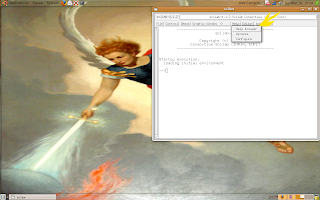
I've developed a prototype of my Mastering project, called SIRENE (acronym in Portuguese).
This project is a system of gesture recognition for the LIBRAS' (Brazilian Sign Language) signs.
This system can be used with any set of gestures made with hands.
The following video was made for an event (here), and I presented it there.
The word "Gravando" means Recording and "Testando" means Testing.
The system that I'm studying is able to recognize 26 gestures, but this prototype is able to recognize only 5 ones.
Of course, this prototype was developed using Scilab and the toolbox SIVp.
Wednesday, December 2, 2009
Thursday, November 5, 2009
More frequencies in FFT
Hi Transmogrifox, thank you very much for your help. We have this blog to interact and to help ourselves.
The Transmogrifox's code is given following:
//Frequency components of a signal
//----------------------------------
// build a noides signal sampled at 1000hz containing to pure frequencies
// at 50 and 70 Hz
sample_rate=1000;
t = 0:1/sample_rate:0.6;
N=size(t,'*'); //number of samples
s=sin(2*%pi*50*t)+ 0.3*sin(2*%pi*70*t+%pi/4)+ 0.2*grand(1,N,'nor',0,1);
y=fft(s);
//the fft response is symetric we retain only the first N/2 points
f=sample_rate*(0:(N/2))/N; //associated frequency vector
n=size(f,'*')
yy = y*2/N;
clf()
plot2d(f,abs(yy(1:n)))
And the following picture is the result.
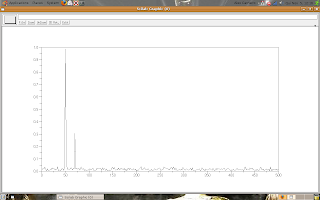
So, if anyone has any question, I think I and Transmogrifox are ready for help.
The Transmogrifox's code is given following:
//Frequency components of a signal
//----------------------------
// build a noides signal sampled at 1000hz containing to pure frequencies
// at 50 and 70 Hz
sample_rate=1000;
t = 0:1/sample_rate:0.6;
N=size(t,'*'); //number of samples
s=sin(2*%pi*50*t)+ 0.3*sin(2*%pi*70*t+%pi/4)+ 0.2*grand(1,N,'nor',0,1);
y=fft(s);
//the fft response is symetric we retain only the first N/2 points
f=sample_rate*(0:(N/2))/N; //associated frequency vector
n=size(f,'*')
yy = y*2/N;
clf()
plot2d(f,abs(yy(1:n)))
And the following picture is the result.
So, if anyone has any question, I think I and Transmogrifox are ready for help.
Tuesday, October 27, 2009
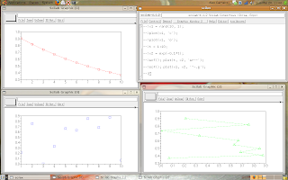
Response in frequency
Hi Cek, I saw your comment (here), and I'd like to say that I never worked with these functions before. But we can learn about the functions.
Let's start with the freq(.) function.
This code is the example in Scilab's help.
s = poly(0, 's');
sys = (s+1)/(s^3-5*s+4);
rep = freq(sys("num"), sys("den"), [0,0.9,1.1,2,3,10,20]);
[horner(sys, 0), horner(sys, 20)]
//
Sys = tf2ss(sys);
[A, B, C, D] = abcd(Sys);
freq(A, B, C, [0, 0.9, 1.1, 2, 3, 10, 20])
In the code, we see the function freq(.) is used with polynomials (in the Space of Laplace). The last argument (the vector [0, 0.9, 1.1, 2, 3, 10, 20]) represents the calculated frequencies for the polynomial sys.
The function tf2ss(.) means time/frequency to state-space.
The function refreq(.) does the same things of the function freq(.), but it uses other arguments.
Look the function's description, in Scilab's help.
[ [frq,] repf] = repfreq(sys, fmin, fmax [, step])
[ [frq,] repf] = repfreq(sys [, frq])
[ frq, repf, splitf] = repfreq(sys, fmin, fmax [, step])
[ frq, repf, splitf] = repfreq(sys [, frq])
sys: syslin list : SIMO linear system
fmin, fmax: two real numbers (lower and upper frequency bounds)
frq: real vector of frequencies (Hz)
step: logarithmic discretization step
splitf: vector of indexes of critical frequencies.
repf: vector of the complex frequency response
The function horner(.) evaluates a polynomial in a specific point, for example:
s = poly(0,'s');
M = [s, 1/s]; // M is the polynomial in analysis
x1 = horner(M,1)
x1
x1 =
1. 1.
x2 = horner(M,%i)
x2 =
i - i
x3 = horner(M,1/s)
x3 =
1 s
- -
s 1
If you want, then we can try to learn anything about the others functions: bode, syslin and csim.
Let's start with the freq(.) function.
This code is the example in Scilab's help.
s = poly(0, 's');
sys = (s+1)/(s^3-5*s+4);
rep = freq(sys("num"), sys("den"), [0,0.9,1.1,2,3,10,20]);
[horner(sys, 0), horner(sys, 20)]
//
Sys = tf2ss(sys);
[A, B, C, D] = abcd(Sys);
freq(A, B, C, [0, 0.9, 1.1, 2, 3, 10, 20])
In the code, we see the function freq(.) is used with polynomials (in the Space of Laplace). The last argument (the vector [0, 0.9, 1.1, 2, 3, 10, 20]) represents the calculated frequencies for the polynomial sys.
The function tf2ss(.) means time/frequency to state-space.
The function refreq(.) does the same things of the function freq(.), but it uses other arguments.
Look the function's description, in Scilab's help.
[ [frq,] repf] = repfreq(sys, fmin, fmax [, step])
[ [frq,] repf] = repfreq(sys [, frq])
[ frq, repf, splitf] = repfreq(sys, fmin, fmax [, step])
[ frq, repf, splitf] = repfreq(sys [, frq])
Parameters
sys: syslin list : SIMO linear system
fmin, fmax: two real numbers (lower and upper frequency bounds)
frq: real vector of frequencies (Hz)
step: logarithmic discretization step
splitf: vector of indexes of critical frequencies.
repf: vector of the complex frequency response
The function horner(.) evaluates a polynomial in a specific point, for example:
s = poly(0,'s');
M = [s, 1/s]; // M is the polynomial in analysis
x1 = horner(M,1)
x1
x1 =
1. 1.
x2 = horner(M,%i)
x2 =
i - i
x3 = horner(M,1/s)
x3 =
1 s
- -
s 1
If you want, then we can try to learn anything about the others functions: bode, syslin and csim.
Friday, October 23, 2009
Operations element by element, again
Hi Jackmatze, how are you? I think you are just as old as me, but it's other thing.
About your question, I made a post that answers you: it's here.
So, let me show an example:
-->matrix1 = [1 2 1;
-->2 1 2;
-->1 2 3]
matrix1 =
1. 2. 1.
2. 1. 2.
1. 2. 3.
-->matrix2 = [1 1 2;
-->0 2 1;
-->1 3 1]
matrix2 =
1. 1. 2.
0. 2. 1.
1. 3. 1.
-->matrix_t = matrix1*matrix2
matrix_t =
2. 8. 5.
4. 10. 7.
4. 14. 7.
-->matrix_dott = matrix1.*matrix2
matrix_dott =
1. 2. 2.
0. 2. 2.
1. 6. 3.
Now, what's the difference of matrix1^2 and matrix1.^2?
matrix1^2 = matrix1*matrix1
matrix1.^2 = matrix1.*matrix1
Ok, Jack? Anything more, I'll try to help you.
Peaks in FFT transformation
Hi Kaustubh, excuse me for the time of the answer.
Do you want to know about the peaks in the FFT transformation (here), right?
Well, this blog is about Scilab, and you can find what you want in any book of Digital Signal Processing.
But God loves you and I'll try to explain what the peaks mean.
Think in a pure frequency signal x(t) like a sine or cosine, it has only the own frequency (f0). The FFT transform is two impulses (X(f) = d(-f0) + d(f0)) (similar to this figure)
If you plot the FFT transform of x(t), then you obtain the peaks in -f0 and f0.
Now, think in a signal composed by two pure frequency signals, y(t) = x1(t) + x2(t), of different frequencies (f1 and f2).
The FFT transform of y(t) is four impulses, two for x1(t) and two for x2(t).
If x1(t) and x2(t) have different amplitudes, for example: x1(t) = cos(2t) and x2(t) = 3 cos(5t), then the peaks of the FFT transform of y(t) are weighted,
Following the example, the FFT transform of x1(t) is X1(f) = d(-f1) + d(f1) and the FFT transformation of x2(t) is X2(t) = 3(d(-f2) + d(f2)). So, the FFT transform of y(t) = x1(t) + x2(t) is Y(f) = X1(f) + X2(f) = (d(-f1) + d(f1)) + 3(d(-f2) + d(f2)).
Now, if you have a real signal xr(t), it has many frequencies and it FFT transform XR(f) presents many peaks, one by each frequency. The peaks' amplitude represents the amplitude of each frequency in xr(t).
My friend, I said this not a blog about Signal Processing, but I tried to help you.
If you have more question, I'll try to help you again.
Tuesday, October 20, 2009
Tensors
Hi Michele, how are you?
First, I'm sorry because I'm not an expert in multi linear algebra and I don't know many things about tensors.
In a fast search, I saw tensors are like matrices with high dimensionality.
Correct me if I were wrong.
tensor1 = zeros(3, 3, 3); // it's a tensor
tensor2 = ones(5, 5, 4); // it's other tensor
I found one function that works with tensors: kron(.). It returns the Kronecker tensor product of two matrices A and B.
The function kron(.) is called like following:
A=[1,2;3,4];
kron(A,A)
ans =
1. 2. 2. 4.
3. 4. 6. 8.
3. 6. 4. 8.
9. 12. 12. 16.
A.*.A // this operator (.*.) implements the Kronecker tensor product of two matrices, look the results are the same kron(A, A) == A.*.A
ans =
1. 2. 2. 4.
3. 4. 6. 8.
3. 6. 4. 8.
9. 12. 12. 16.
I think it's something about tensors.
If anyone has a comment or suggestion, I ask for you share your knowledge with us.
Thursday, October 8, 2009
Topics of Digital Image Processing
Hi Wahlau, I saw your comment but I couldn't answer it before. Thank you for your words to me.
I have another blog and I made some posts about Image Processing and Segmentation (in Portuguese).
If you want to develop anything like the interactive ball, then you should learn about skin segmentation and how to interact the virtual ball with the segmented region.
The simplest algorithm for skin segmentation is the threshold in the channels of color Cb and Cr (in images coded in YCbCr).
The toolbox SIVp has functions for read, write, show, convert, and others operations with images. That toolbox is too simple for install, if you use GNU/Linux, you can install it using the apt-get or synaptic.
PS.: In my other blog, I posted some codes in Scilab for skin segmentation, and anything more.
Tuesday, October 6, 2009
Excuses
Hi Stanley and Naza, I'm sorry I couldn't answer your questions because I'm writing my dissertation and I needed to make two articles too.
So, I ask for you explain better what you want.
Stanley, I think the meshgrid() function can help you, like following:
N = 20;
x_range = -1:2/(N - 1):1;
y_range = -1:1.2/(N - 1):0.2;
[x y] = meshgrid(x_range, y_range);
P = [];
for i1 = 1:N,
for i2 = 1:N,
P(i2,i1) = color_P(i1, i2); //here you put the function P = f(x, y)
end;
end;
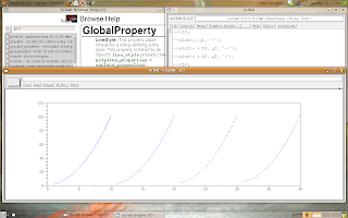
For plot the graph, you can use the fplot3d1(.) function. The following picture shows a example:
deff('z=f(x,y)','z=x^4-y')
x=-3:0.2:3 ;y=x ;
fplot3d1(x, y, f, alpha = 0, theta = 0); // alpha and theta are the rotation angles
The result is:
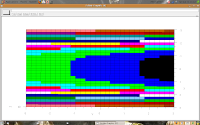
Now, you study the fplot3d1(.) function for make your own graph.
The presented function plots graphs as surfaces if you change the variables alpha and theta (try alpha = 5 and theta = 30).
That's all.
So, I ask for you explain better what you want.
Stanley, I think the meshgrid() function can help you, like following:
N = 20;
x_range = -1:2/(N - 1):1;
y_range = -1:1.2/(N - 1):0.2;
[x y] = meshgrid(x_range, y_range);
P = [];
for i1 = 1:N,
for i2 = 1:N,
P(i2,i1) = color_P(i1, i2); //here you put the function P = f(x, y)
end;
end;
---------------
For plot the graph, you can use the fplot3d1(.) function. The following picture shows a example:
deff('z=f(x,y)','z=x^4-y')
x=-3:0.2:3 ;y=x ;
fplot3d1(x, y, f, alpha = 0, theta = 0); // alpha and theta are the rotation angles
The result is:

Now, you study the fplot3d1(.) function for make your own graph.
The presented function plots graphs as surfaces if you change the variables alpha and theta (try alpha = 5 and theta = 30).
That's all.
Thursday, October 1, 2009
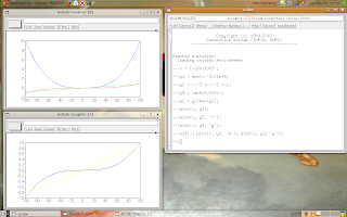
Digital Signal Processing - intro
Hi Wallace, I'd like to know what algorithm, or kind of algorithm, you need to develop.
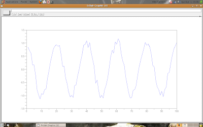
I made a post about convolution, but I think it's a good, and simple, subject for we start our studies.
Look the noised signal:
-->T = 100;
-->t = 1:T;
-->w = %pi/10;
-->s = cos(w*t); //pure signal
-->n = rand(1, T, 'normal')*0.1; //noise
-->x = s + n;
-->plot(t, x);
The result is:
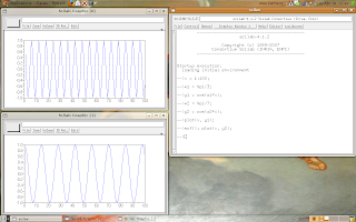
Now, let's filter the signal using an average filter.
We have two options for apply the filtering:
-->Tm = 5;
-->y = [];
-->for i = 1:Tm,
-->y(i) = mean(x(1:i));
-->end;
-->for i = (Tm + 1):T,
-->y(i) = mean(x((i - Tm):i));
-->end;
-->plot(t, y);
The result is:

-->Tm = 5;
-->m = ones(1, Tm);
-->y = convol(x, m);
-->ty = 1:length(y);
-->plot(ty, y);
The result is:
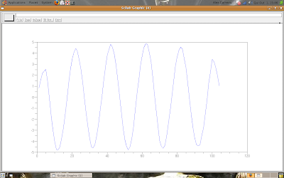
If you make the math operations, you'll see the results are, numerically, the same for t = Tm + 1 until t = T.
I made a post about convolution, but I think it's a good, and simple, subject for we start our studies.
Look the noised signal:
-->T = 100;
-->t = 1:T;
-->w = %pi/10;
-->s = cos(w*t); //pure signal
-->n = rand(1, T, 'normal')*0.1; //noise
-->x = s + n;
-->plot(t, x);
The result is:

Now, let's filter the signal using an average filter.
We have two options for apply the filtering:
The first
-->Tm = 5;
-->y = [];
-->for i = 1:Tm,
-->y(i) = mean(x(1:i));
-->end;
-->for i = (Tm + 1):T,
-->y(i) = mean(x((i - Tm):i));
-->end;
-->plot(t, y);
The result is:

The second
-->Tm = 5;
-->m = ones(1, Tm);
-->y = convol(x, m);
-->ty = 1:length(y);
-->plot(ty, y);
The result is:

If you make the math operations, you'll see the results are, numerically, the same for t = Tm + 1 until t = T.
Tuesday, September 22, 2009
For my readers
I thought my readers will like to know the videos, in the last post, but nobody made any comment.
So, I thought my readers should choose the next subject.
I think the basic commands are well presented here.
I'd like to propose some subjects:
So, I thought my readers should choose the next subject.
I think the basic commands are well presented here.
I'd like to propose some subjects:
- Digital image processing
- Digital signal processing
- Advanced Graphs
- Advanced algebraic manipulations
Thursday, September 10, 2009
Videos in YouTube
I was looking my YouTube's account today, and I saw some videos that I made using Scilab.
If anyone wants to see the videos, this is my Channel in YouTube: http://www.youtube.com/alexsheep7
Following two great videos.
If anyone wants to see the videos, this is my Channel in YouTube: http://www.youtube.com/alexsheep7
Following two great videos.
A simple code that shows graphs.
A more complex code that implements extended reality.
Monday, September 7, 2009
Discrete convolution properties - 2
Anyone called Younes asked something about convolution via Fourier Transform.
I made the following deduction for you Younes (click on the image for see it in the real size):
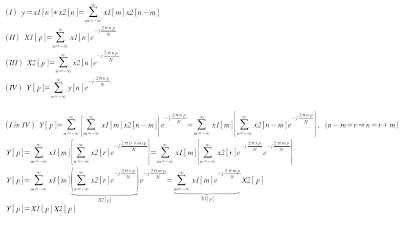
Now, I ask: try to confirm the property using Scilab.
Don't forget computers don't make infinity operations.
I made the following deduction for you Younes (click on the image for see it in the real size):

Now, I ask: try to confirm the property using Scilab.
Don't forget computers don't make infinity operations.
Saturday, August 29, 2009
Discrete convolution properties - 1
I received a comment here. And, this post is about discrete convolution properties.
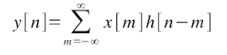
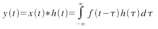
The continuous form of the convolution is given by:

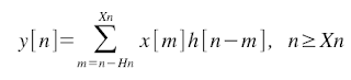
So, the discrete form is given by:
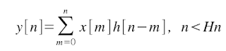
If x[n] and h[n] are limited in the time ({x[n] = 0 if n <> Xn} and {h[n] = 0 if n <> Hn}), then the convolution is implemented as follow:
Let's suppose Xn > Hn (if Hn > Xn, the analysis is the same).
The equation is separated in three cases:
Case 1
 Case 2
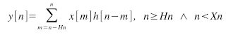 Case 3
 Any other situation, y[n] = 0.
If you make an analysis in y[n], you'll see that y[n] = 0, if n <> Xn + Hn - 1.
Some other properties of the discrete convolution are the same than the continuous convolution:
Say me what happens.
The continuous form of the convolution is given by:

So, the discrete form is given by:

If x[n] and h[n] are limited in the time ({x[n] = 0 if n <> Xn} and {h[n] = 0 if n <> Hn}), then the convolution is implemented as follow:
Let's suppose Xn > Hn (if Hn > Xn, the analysis is the same).
The equation is separated in three cases:
Case 1
 Case 2
 Case 3
 Any other situation, y[n] = 0.
If you make an analysis in y[n], you'll see that y[n] = 0, if n <> Xn + Hn - 1.
Some other properties of the discrete convolution are the same than the continuous convolution:
- x[n] * h[n] = h[n] * x[n];
- x[n]*(h1[n]*h2[n]) = (x[n]*h1[n])*h2[n];
- x[n]*(h1[n] + h2[n]) = x[n]*h1[n] + x[n]*h2[n];
- a(x[n]*h[n]) = (ax[n])*h[n] = x[n]*(ah[n]), a is real;
- x[n]*d[n] = x[n], d[n] = 1 if n = 0 and d[n] = 0 if n is not null;
- x[n]*xi[n] = d[n], xi[n] is the inverse of x[n].
Say me what happens.
Tuesday, August 25, 2009
Basic statistic
Hi Naza, I saw your comment and I'll make your post soon.
In this post, I want to teach something about basic statistic.
I recommend the Papoulis' book for who intends to study statistic.
Here, I'd like to write about random variables and some operations.
A random variable is a variable that you don't know it value.
In Scilab, random variables are created by the rand(.) function.
The default distribution of probability used in the rand(.) function is uniform (between [0, 1]), but the function supports the normal distribution (with null mean and unitary variance) too.
An example:
x1 = rand()
x1 =
0.5608486
x2 = rand(1, 1, 'uniform') // one line and one column (a scalar variable)
x2 =
0.6623569
x3 = rand(1, 1, 'normal')
x3 =
0.6380837
If you have many values in a variable, like this:
x = rand(10, 1); // ten lines and one column
x =
0.3616361
0.2922267
0.5664249
0.4826472
0.3321719
0.5935095
0.5015342
0.4368588
0.2693125
0.6325745
then you can see the histogram using the histplot(.) function.
histplot(5, x); // the function takes the biggest and the smallest values, divides the interval in five parts (the number 5, first argument), and counts how many numbers are in each part
Look the result:
Now, let's do a smarter example:
x = rand(10000, 1);
y = 10*x + 2;
histplot(20, x);
scf(); histplot(20, y);
Look the result:
The graphs look like the same, but if you click over the image then you can see the indexes.
The left graph (variable x) has the indexes in the interval [0, 1] and the right graph (variable y) has the indexes in the interval [2, 12].
I ask to my readers: why the indexes are these?
In this post, I want to teach something about basic statistic.
I recommend the Papoulis' book for who intends to study statistic.
Here, I'd like to write about random variables and some operations.
A random variable is a variable that you don't know it value.
In Scilab, random variables are created by the rand(.) function.
The default distribution of probability used in the rand(.) function is uniform (between [0, 1]), but the function supports the normal distribution (with null mean and unitary variance) too.
An example:
x1 = rand()
x1 =
0.5608486
x2 = rand(1, 1, 'uniform') // one line and one column (a scalar variable)
x2 =
0.6623569
x3 = rand(1, 1, 'normal')
x3 =
0.6380837
If you have many values in a variable, like this:
x = rand(10, 1); // ten lines and one column
x =
0.3616361
0.2922267
0.5664249
0.4826472
0.3321719
0.5935095
0.5015342
0.4368588
0.2693125
0.6325745
then you can see the histogram using the histplot(.) function.
histplot(5, x); // the function takes the biggest and the smallest values, divides the interval in five parts (the number 5, first argument), and counts how many numbers are in each part
Look the result:

Now, let's do a smarter example:
x = rand(10000, 1);
y = 10*x + 2;
histplot(20, x);
scf(); histplot(20, y);
Look the result:

The graphs look like the same, but if you click over the image then you can see the indexes.
The left graph (variable x) has the indexes in the interval [0, 1] and the right graph (variable y) has the indexes in the interval [2, 12].
I ask to my readers: why the indexes are these?
Monday, August 17, 2009
Convolution
I wrote a post about convolution in my other blog, but I'll write here how to use the convolution in Scilab.
The convolution is a operation with two functions defined as:
The function in Scilab that implements the convolution is convol(.).
Let's do the test: I'll convolve a cosine (five periods) with itself (one period):
N1 = 100;
N2 = 20;
n1 = 1:N1;
n2 = 1:N2;
w = %pi/10;
f1 = cos(w*n1);
f2 = cos(w*n2);
y = convol(f1, f2);
plot(f1);
scf(); plot(f2);
scf(); plot(y);
The result is:
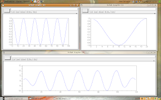
The top left graph is f1, the top right is f2 and the bottom graph is y.
Again, if anyone wants, I can write about discrete convolution properties.
The convolution is a operation with two functions defined as:

The function in Scilab that implements the convolution is convol(.).
Let's do the test: I'll convolve a cosine (five periods) with itself (one period):
N1 = 100;
N2 = 20;
n1 = 1:N1;
n2 = 1:N2;
w = %pi/10;
f1 = cos(w*n1);
f2 = cos(w*n2);
y = convol(f1, f2);
plot(f1);
scf(); plot(f2);
scf(); plot(y);
The result is:

The top left graph is f1, the top right is f2 and the bottom graph is y.
Again, if anyone wants, I can write about discrete convolution properties.
Monday, August 10, 2009
FFT - specifying the frequencies
I'd like to know my readers, but the "no name" readers deserve respect, as everybody.
This post is about the FFT function, and anyone wants to know how to specify the frequencies for plot the values.
A few of theory:
If your signal has N values [0, N - 1], then the Fourier Transform has N distinct values.
The function fft(.) returns the signal in the interval [0, N - 1], so you can use the function fftshift(.), over the function fft(.) like this: X = fftshift(fft(x)), that it returns the Fourier Transform in the intervals:
About the frequencies, if your signal was sampled with a rate T (T samples by second), the indexes are given multiplying the interval by: 2*%pi*T.
Look the example:
N = 100;
n = 1:N;
T = 0.1; // one sample by each 0.1s
w = 0.5; // frequency of the sampled signal (in radians)
x = cos(w*n);
plot(n*T, x); // plot the signal indexed by seconds
f = [-N/2:N/2 - 1];
X = fftshift(fft(x));
scf();
plot(f*2*%pi*T, X); // plot the signal indexed by radians
The result is:
Observing that w = 0.5 is the frequency of the sampled signal, the true frequency (of the analog source signal) is given by w_source = w/T = 0.5/0.1 = 5 rad/s. Now, click on the image and look where the peaks are.
This post is about the FFT function, and anyone wants to know how to specify the frequencies for plot the values.
A few of theory:
If your signal has N values [0, N - 1], then the Fourier Transform has N distinct values.
The function fft(.) returns the signal in the interval [0, N - 1], so you can use the function fftshift(.), over the function fft(.) like this: X = fftshift(fft(x)), that it returns the Fourier Transform in the intervals:
- [-(N - 1)/2, (N - 1)/2], if N is odd.
- [-N/2, N/2 - 1], if N is even.
About the frequencies, if your signal was sampled with a rate T (T samples by second), the indexes are given multiplying the interval by: 2*%pi*T.
Look the example:
N = 100;
n = 1:N;
T = 0.1; // one sample by each 0.1s
w = 0.5; // frequency of the sampled signal (in radians)
x = cos(w*n);
plot(n*T, x); // plot the signal indexed by seconds
f = [-N/2:N/2 - 1];
X = fftshift(fft(x));
scf();
plot(f*2*%pi*T, X); // plot the signal indexed by radians
The result is:

Observing that w = 0.5 is the frequency of the sampled signal, the true frequency (of the analog source signal) is given by w_source = w/T = 0.5/0.1 = 5 rad/s. Now, click on the image and look where the peaks are.
Wednesday, August 5, 2009
Making functions
A important resource in any programming language is to make specific functions.
Using Scilab we may make our own functions.
For example, if we need a function that adds two numbers and divides the result by two, we can call that function as add_d2(v1, v2).
The follow script is made in the editor.
function [result] = add_d2(v1, v2)
aux = v1 + v2;
result = aux/2;
endfunction;
Or, we can write just one line of code:
function [result] = add_d2(v1, v2)
result = (v1 + v2)/2;
endfunction;
Obvious, the example is too simple, but I'd like to give a example for present the syntax.
Ok, let's make a better example:
We need a function that finds the peaks in a signal and returns two variable, one with the position and the other with the value of each peak.
function [positions, values] = find_peaks(x)
positions = [];
values = [];
n_peaks = 0;
for i = 2:length(x) - 1, // x should be a vector, like: x = [x_1 x_2 x_3 ... x_n]
if (x(i) > x(i - 1)) & (x(i) > x(i + 1)),
n_peaks = n_peaks + 1;
positions(n_peaks) = i;
values(n_peaks) = x(i);
end;
end;
endfunction;
Test the code and say me what happens.
Saturday, August 1, 2009
Fast Fourier Transform - FFT
This post is about a good subject in many areas of engineering and informatics: the Fourier Transform. The continuous Fourier Transform is defined as:
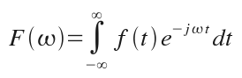
f(t) is a continuous function and F(w) is the Fourier Transform of f(t).
But, the computers don't work with continuous functions, so we should use the discrete form of the Fourier Transform:
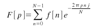
f[n] is a discrete function of N elements, F[p] is a discrete and periodic function of period N, so we calculate just N (0 to N - 1) elements for F[p].
Who studies digital signal processing or instrumentation and control knows the utilities of this equation.
Now, how to use the Fourier Transform in Scilab?
If we are using large signals, like audio files, the discrete Fourier Transform is not a good idea, then we can use the fast Fourier Transform (used with discrete signals), look the script:
-->N = 100; // number of elements of the signal
-->n = 0:N - 1;
-->w1 = %pi/5; // 1st frequency
-->w2 = %pi/10; // 2nd frequency
-->s1 = cos(w1*n); // 1st component of the signal
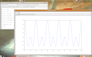
-->s2 = cos(w2*n); // 2nd component of the signal
-->f = s1 + s2; // signal
-->plot(n, f);
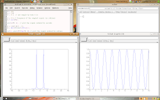
The result is:
Now, let's study the Fourier Transform of our signal.
-->F = fft(f); // it calculates the Fourier Transform
-->F_abs = abs(F); // F_abs is the absolute value of each element of F
-->plot(n, F_abs);
The result is:
The Fourier Transform is a linear transformation, thus it has a inverse transformation: the Inverse Fourier Transform.
Scilab has the function ifft(.) for obtain the original signal from it Fourier Transform.
If anyone wants to know, I can make a new post about how to identify the frequencies of the original signal in the Fourier Transform.

f(t) is a continuous function and F(w) is the Fourier Transform of f(t).
But, the computers don't work with continuous functions, so we should use the discrete form of the Fourier Transform:

f[n] is a discrete function of N elements, F[p] is a discrete and periodic function of period N, so we calculate just N (0 to N - 1) elements for F[p].
Who studies digital signal processing or instrumentation and control knows the utilities of this equation.
Now, how to use the Fourier Transform in Scilab?
If we are using large signals, like audio files, the discrete Fourier Transform is not a good idea, then we can use the fast Fourier Transform (used with discrete signals), look the script:
-->N = 100; // number of elements of the signal
-->n = 0:N - 1;
-->w1 = %pi/5; // 1st frequency
-->w2 = %pi/10; // 2nd frequency
-->s1 = cos(w1*n); // 1st component of the signal
-->s2 = cos(w2*n); // 2nd component of the signal
-->f = s1 + s2; // signal
-->plot(n, f);
The result is:

Now, let's study the Fourier Transform of our signal.
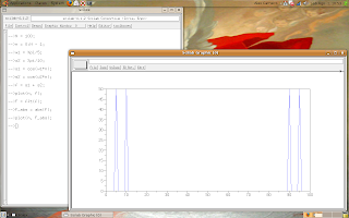
-->F = fft(f); // it calculates the Fourier Transform
-->F_abs = abs(F); // F_abs is the absolute value of each element of F
-->plot(n, F_abs);
The result is:

Look at the two graph's peaks, one for the component s1 and the other for the component s2.
The Fourier Transform is a linear transformation, thus it has a inverse transformation: the Inverse Fourier Transform.
Scilab has the function ifft(.) for obtain the original signal from it Fourier Transform.
If anyone wants to know, I can make a new post about how to identify the frequencies of the original signal in the Fourier Transform.
Wednesday, July 29, 2009
Color vectors
I received a comment (here) asking about color in plotting vectors.
Ok, I'd not write about properties of figures but the reader's satisfaction is more important.
We can manipulate any property of the graphs in Scilab as following:
--> set("figure_style","new"); //create a figure in entity mode
-->f = get("current_figure")
f =
Handle of type "Figure" with properties:
========================================
children: "Axes"
figure_style = "new"
figure_position = [655,473]
figure_size = [610,461]
axes_size = [596,397]
auto_resize = "on"
figure_name = "Scilab Graphic (%d)"
figure_id = 0
color_map= matrix 32x3
pixmap = "off"
pixel_drawing_mode = "copy"
immediate_drawing = "on"
background = -2
visible = "on"
rotation_style = "unary"
user_data = []
--> a = f.children // the handle on the Axes child
Now, let's set the desired color:
--> a.foreground = 5;
And we can make the graph:
--> x = [1:10]';
--> y = [1:10]';
--> [vx vy] = meshgrid(x, y);
--> champ(x, y, vx, vy, 1);
The result is:
But, we want more! Let's continue the script as following:
--> a.foreground = 3;
--> x = 10 + [1:10]';
--> y = 10 + [1:10]';
--> [vx vy] = meshgrid(x, y);
--> champ(x, y, vx, vy, 1);
The result is:
The foreground element, called in
--> a.foreground = n; // n is a number that represents the desired color
may be any of these values:
Scilab can make graphs with more colors (for the numbers higher or equal than 10), but you are smart for test it.
If you want a black bound (look that the made graphs, the bound's color is the same of the vectors) you have to put the command
--> a.foreground = 1;
after the champ(.) function:
That's all, now the unknown reader can plot vectors with colors.
Ok, I'd not write about properties of figures but the reader's satisfaction is more important.
We can manipulate any property of the graphs in Scilab as following:
--> set("figure_style","new"); //create a figure in entity mode
-->f = get("current_figure")
f =
Handle of type "Figure" with properties:
========================================
children: "Axes"
figure_style = "new"
figure_position = [655,473]
figure_size = [610,461]
axes_size = [596,397]
auto_resize = "on"
figure_name = "Scilab Graphic (%d)"
figure_id = 0
color_map= matrix 32x3
pixmap = "off"
pixel_drawing_mode = "copy"
immediate_drawing = "on"
background = -2
visible = "on"
rotation_style = "unary"
user_data = []
--> a = f.children // the handle on the Axes child
Now, let's set the desired color:
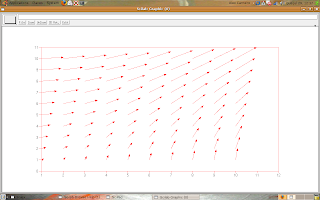
--> a.foreground = 5;
And we can make the graph:
--> x = [1:10]';
--> y = [1:10]';
--> [vx vy] = meshgrid(x, y);
--> champ(x, y, vx, vy, 1);
The result is:

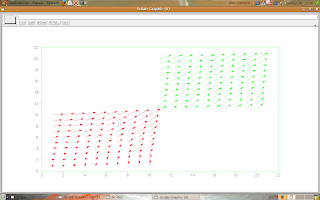
But, we want more! Let's continue the script as following:
--> a.foreground = 3;
--> x = 10 + [1:10]';
--> y = 10 + [1:10]';
--> [vx vy] = meshgrid(x, y);
--> champ(x, y, vx, vy, 1);
The result is:

The foreground element, called in
--> a.foreground = n; // n is a number that represents the desired color
may be any of these values:
- 1 - black
- 2 - blue
- 3 - green
- 4 - cyan
- 5 - red
- 6 - magenta
- 7 - yellow
- 8 - white
- 9 - dark blue
Scilab can make graphs with more colors (for the numbers higher or equal than 10), but you are smart for test it.
If you want a black bound (look that the made graphs, the bound's color is the same of the vectors) you have to put the command
--> a.foreground = 1;
after the champ(.) function:
That's all, now the unknown reader can plot vectors with colors.
Wednesday, July 22, 2009
Lists in Scilab
Hi everybody, I couldn't post anything last week because I was in a retreat.
Let's study something about lists in Scilab now.
Lists are a type of variables like vectors, but each element may be of any type.
In vectors, all elements are of the same type (vectors of integers, doubles, strings, etc...).
In lists, we may have many types of variables.
Creating a list:
Scilab has a function called list(.) and it may be used with any quantity of elements. Look the examples:
-->person1 = list("Josh", 25, 1.8, 80, "soccer");
-->person2 = list("Mary", 22, 1.6, 55, "tennis");
-->person3 = list("Peter", 30, 1.75, 100, "chess");
-->person1
person1 =
person1(1)
Josh
person1(2)
25.
person1(3)
1.8
person1(4)
80.
person1(5)
soccer
-->person2
person2 =
person2(1)
Mary
person2(2)
22.
person2(3)
1.6
person2(4)
55.
person2(5)
tennis
-->person3
person3 =
person3(1)
Peter
person3(2)
30.
person3(3)
1.75
person3(4)
100.
person3(5)
chess
Each person has five informations:
But, if we want to insert more informations, then we can do:
-->person1($ + 1) = "male"
person1 =
person1(1)
Josh
person1(2)
25.
person1(3)
1.8
person1(4)
80.
person1(5)
soccer
person1(6)
male
-->person2($ + 1) = "female"
person2 =
person2(1)
Mary
person2(2)
22.
person2(3)
1.6
person2(4)
55.
person2(5)
tennis
person2(6)
female
-->person3($ + 1) = "male"
person3 =
person3(1)
Peter
person3(2)
30.
person3(3)
1.75
person3(4)
100.
person3(5)
chess
person3(6)
male
The indexes may be manipulated for insert new elements in any point of the list.
If anyone has any question about lists (or others subjects), I can try to answer.
Let's study something about lists in Scilab now.
Lists are a type of variables like vectors, but each element may be of any type.
In vectors, all elements are of the same type (vectors of integers, doubles, strings, etc...).
In lists, we may have many types of variables.
Creating a list:
Scilab has a function called list(.) and it may be used with any quantity of elements. Look the examples:
-->person1 = list("Josh", 25, 1.8, 80, "soccer");
-->person2 = list("Mary", 22, 1.6, 55, "tennis");
-->person3 = list("Peter", 30, 1.75, 100, "chess");
-->person1
person1 =
person1(1)
Josh
person1(2)
25.
person1(3)
1.8
person1(4)
80.
person1(5)
soccer
-->person2
person2 =
person2(1)
Mary
person2(2)
22.
person2(3)
1.6
person2(4)
55.
person2(5)
tennis
-->person3
person3 =
person3(1)
Peter
person3(2)
30.
person3(3)
1.75
person3(4)
100.
person3(5)
chess
Each person has five informations:
- Name
- Age
- Height
- Weight
- Favorite sport
But, if we want to insert more informations, then we can do:
-->person1($ + 1) = "male"
person1 =
person1(1)
Josh
person1(2)
25.
person1(3)
1.8
person1(4)
80.
person1(5)
soccer
person1(6)
male
-->person2($ + 1) = "female"
person2 =
person2(1)
Mary
person2(2)
22.
person2(3)
1.6
person2(4)
55.
person2(5)
tennis
person2(6)
female
-->person3($ + 1) = "male"
person3 =
person3(1)
Peter
person3(2)
30.
person3(3)
1.75
person3(4)
100.
person3(5)
chess
person3(6)
male
The indexes may be manipulated for insert new elements in any point of the list.
If anyone has any question about lists (or others subjects), I can try to answer.
Tuesday, July 7, 2009
A car and a truck
What's the difference between a car and a truck?
Scilab explains it! Look the Scilab's example video:
Open the window of examples (demonstrations) clicking the Demos button, so you can try all the examples.
Scilab explains it! Look the Scilab's example video:
Open the window of examples (demonstrations) clicking the Demos button, so you can try all the examples.
Monday, June 29, 2009
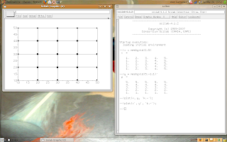
Some examples
I made a video with some examples.
Look that the Scilab presents the example's codes.
If the readers like my initiative, then I can make more videos.
Look that the Scilab presents the example's codes.
If the readers like my initiative, then I can make more videos.
Friday, June 26, 2009
Polynomials
Let's learn something different today.
We study polynomials at school, so we are going to learn anything about how Scilab works with them.
First, this post is moved to fractions of polynomials, for example*:
For work with polynomials in Scilab, we use the %s as the variable. Look the example**:
-->A = %s^2 + %s + 1
A =
2
1 + s + s
-->B = %s + 2
B =
2 + s
-->R = A*B
R =
2 3
2 + 3s + 3s + s
-->Q = A/B
Q =
2
1 + s + s
---------
2 + s
-->S = A + B
S =
2
3 + 2s + s
-->D = A - B
D =
2
- 1 + s
Observe that Scilab works correctly with the coefficients.
Now, let's work more, if we have a fraction of polynomials and we need just the denominator:
-->Q = (%s + 1)/(%s^2 + 2*%s + 2)
Q =
1 + s
---------
2
2 + 2s + s
-->Dem = denom(Q)
Dem =
2
2 + 2s + s
Following with the example, now we need just the numerator:
-->Num = numer(Q)
Num =
1 + s
And now, we need the roots of the denominator and of the numerator:
-->R_Dem = roots(Dem)
R_Dem =
- 1. + i
- 1. - i
-->R_Num = roots(Num)
R_Num =
- 1.
If anyone has studied linear systems, post a comment here.
If nobody has studied it, you can make a post too.
-----------------------
* I use OpenOffice Math for create the equations.
** The blog doesn't work with white spaces, but Scilab puts the higher coefficients after.
We study polynomials at school, so we are going to learn anything about how Scilab works with them.
First, this post is moved to fractions of polynomials, for example*:

For work with polynomials in Scilab, we use the %s as the variable. Look the example**:
-->A = %s^2 + %s + 1
A =
2
1 + s + s
-->B = %s + 2
B =
2 + s
-->R = A*B
R =
2 3
2 + 3s + 3s + s
-->Q = A/B
Q =
2
1 + s + s
---------
2 + s
-->S = A + B
S =
2
3 + 2s + s
-->D = A - B
D =
2
- 1 + s
Observe that Scilab works correctly with the coefficients.
Now, let's work more, if we have a fraction of polynomials and we need just the denominator:
-->Q = (%s + 1)/(%s^2 + 2*%s + 2)
Q =
1 + s
---------
2
2 + 2s + s
-->Dem = denom(Q)
Dem =
2
2 + 2s + s
Following with the example, now we need just the numerator:
-->Num = numer(Q)
Num =
1 + s
And now, we need the roots of the denominator and of the numerator:
-->R_Dem = roots(Dem)
R_Dem =
- 1. + i
- 1. - i
-->R_Num = roots(Num)
R_Num =
- 1.
If anyone has studied linear systems, post a comment here.
If nobody has studied it, you can make a post too.
-----------------------
* I use OpenOffice Math for create the equations.
** The blog doesn't work with white spaces, but Scilab puts the higher coefficients after.
Tuesday, June 23, 2009
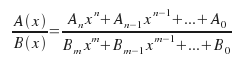
Plot 3D - surface
Ok, the world is learning how to use Scilab. I like it a lot!
Now, let's make surfaces using the function plot3d(.).
This function is called like this: plot3d(x, y, z);
Where x and y are vectors and z is a matrix.
Look the example:
-->d = -3:3;
-->[x y] = meshgrid(d)
y =
- 3. - 3. - 3. - 3. - 3. - 3. - 3.
- 2. - 2. - 2. - 2. - 2. - 2. - 2.
- 1. - 1. - 1. - 1. - 1. - 1. - 1.
0. 0. 0. 0. 0. 0. 0.
1. 1. 1. 1. 1. 1. 1.
2. 2. 2. 2. 2. 2. 2.
3. 3. 3. 3. 3. 3. 3.
x =
- 3. - 2. - 1. 0. 1. 2. 3.
- 3. - 2. - 1. 0. 1. 2. 3.
- 3. - 2. - 1. 0. 1. 2. 3.
- 3. - 2. - 1. 0. 1. 2. 3.
- 3. - 2. - 1. 0. 1. 2. 3.
- 3. - 2. - 1. 0. 1. 2. 3.
- 3. - 2. - 1. 0. 1. 2. 3.
-->z = 9 - (x.^2 + y.^2);
-->plot3d(d, d, z);
The result is showed:
The coordinates x and y were the vector d (-3:3).
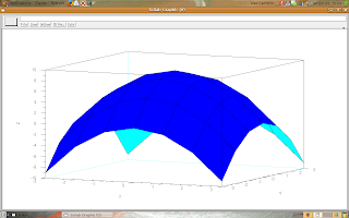
We can make any surface, so let's think in other surface. Look the next example:
-->x = -5:0.1:5;
-->y = 0:0.1:10;
-->[xc yc] = meshgrid(x, y);
-->w = %pi/4;
-->b = -0.5;
-->z = exp(b*yc).*sin(w*xc);
-->plot3d(x, y, z);
The result:
Try to make tests and generate surfaces.
Now, let's make surfaces using the function plot3d(.).
This function is called like this: plot3d(x, y, z);
Where x and y are vectors and z is a matrix.
Look the example:
-->d = -3:3;
-->[x y] = meshgrid(d)
y =
- 3. - 3. - 3. - 3. - 3. - 3. - 3.
- 2. - 2. - 2. - 2. - 2. - 2. - 2.
- 1. - 1. - 1. - 1. - 1. - 1. - 1.
0. 0. 0. 0. 0. 0. 0.
1. 1. 1. 1. 1. 1. 1.
2. 2. 2. 2. 2. 2. 2.
3. 3. 3. 3. 3. 3. 3.
x =
- 3. - 2. - 1. 0. 1. 2. 3.
- 3. - 2. - 1. 0. 1. 2. 3.
- 3. - 2. - 1. 0. 1. 2. 3.
- 3. - 2. - 1. 0. 1. 2. 3.
- 3. - 2. - 1. 0. 1. 2. 3.
- 3. - 2. - 1. 0. 1. 2. 3.
- 3. - 2. - 1. 0. 1. 2. 3.
-->z = 9 - (x.^2 + y.^2);
-->plot3d(d, d, z);
The result is showed:

The coordinates x and y were the vector d (-3:3).
We can make any surface, so let's think in other surface. Look the next example:
-->x = -5:0.1:5;
-->y = 0:0.1:10;
-->[xc yc] = meshgrid(x, y);
-->w = %pi/4;
-->b = -0.5;
-->z = exp(b*yc).*sin(w*xc);
-->plot3d(x, y, z);
The result:

Try to make tests and generate surfaces.
Friday, June 12, 2009
Plotting vectors like an animation
The last post received a comment, so I thought the readers could like to see anything more about how to plot vectors.
Let's use the Scilab's text editor, click the 'Editor' button and write the scripts, look the images.
 Opening the editor.
 Using the editor.
Read the buttons for use the editor's resources.
Now, let's see what happens when the following script is executed:
r = 0.1:0.1:10;
w = %pi/10;
x_i = 0;
y_i = 0;
for t = 1:length(r),
x_f = r(t)*cos(w*t);
y_f = r(t)*sin(w*t);
champ(x_i, y_i, x_f - x_i, y_f - y_i, 0.1);
x_i = x_f;
y_i = y_f;
sleep(100);
end;
--------------
The result:
Friday, June 5, 2009
Plotting vectors
I received an e-mail from a reader, I feel happy with it, so if anyone needs help, I'm receiving asks.
So, let's follow with our Scilab's tutorial.
This post is about plotting vectors, like the picture.

This kind of plotting is very common for applications on electromagnetism or analysis of fluids.
In Scilab, we can use the champ(.) function for plotting vectors.
Look the following script:
-->x = -5:5;
-->y = 0:4;
-->[xv yv] = meshgrid(x, y)
yv =
0. 0. 0. 0. 0. 0. 0. 0. 0. 0. 0.
1. 1. 1. 1. 1. 1. 1. 1. 1. 1. 1.
2. 2. 2. 2. 2. 2. 2. 2. 2. 2. 2.
3. 3. 3. 3. 3. 3. 3. 3. 3. 3. 3.
4. 4. 4. 4. 4. 4. 4. 4. 4. 4. 4.
xv =
- 5. - 4. - 3. - 2. - 1. 0. 1. 2. 3. 4. 5.
- 5. - 4. - 3. - 2. - 1. 0. 1. 2. 3. 4. 5.
- 5. - 4. - 3. - 2. - 1. 0. 1. 2. 3. 4. 5.
- 5. - 4. - 3. - 2. - 1. 0. 1. 2. 3. 4. 5.
- 5. - 4. - 3. - 2. - 1. 0. 1. 2. 3. 4. 5.
-->wx = %pi/3;
-->xv = cos(wx*xv);
-->yv = yv/max(yv);
-->champ(x, y, xv', yv', 1);
The result is showed following:
The champ(.) has five arguments, the first and the second are the coordinates of each vector, the third and the fourth are the components of each vector, and the fifth is a correction argument (for normalization).
Try to make graphs and say me what happens.
So, let's follow with our Scilab's tutorial.
This post is about plotting vectors, like the picture.

This kind of plotting is very common for applications on electromagnetism or analysis of fluids.
In Scilab, we can use the champ(.) function for plotting vectors.
Look the following script:
-->x = -5:5;
-->y = 0:4;
-->[xv yv] = meshgrid(x, y)
yv =
0. 0. 0. 0. 0. 0. 0. 0. 0. 0. 0.
1. 1. 1. 1. 1. 1. 1. 1. 1. 1. 1.
2. 2. 2. 2. 2. 2. 2. 2. 2. 2. 2.
3. 3. 3. 3. 3. 3. 3. 3. 3. 3. 3.
4. 4. 4. 4. 4. 4. 4. 4. 4. 4. 4.
xv =
- 5. - 4. - 3. - 2. - 1. 0. 1. 2. 3. 4. 5.
- 5. - 4. - 3. - 2. - 1. 0. 1. 2. 3. 4. 5.
- 5. - 4. - 3. - 2. - 1. 0. 1. 2. 3. 4. 5.
- 5. - 4. - 3. - 2. - 1. 0. 1. 2. 3. 4. 5.
- 5. - 4. - 3. - 2. - 1. 0. 1. 2. 3. 4. 5.
-->wx = %pi/3;
-->xv = cos(wx*xv);
-->yv = yv/max(yv);
-->champ(x, y, xv', yv', 1);
The result is showed following:

The champ(.) has five arguments, the first and the second are the coordinates of each vector, the third and the fourth are the components of each vector, and the fifth is a correction argument (for normalization).
Try to make graphs and say me what happens.
Tuesday, May 26, 2009
Making a grid
I'm happy with this blog, I received my first comment (here) this week, thank you Naza Sundae.
Following with our online Scilab's tutorial, let's learn how to make grids, like the figure:
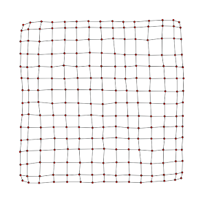 This type of graphs are very important for data visualization.
The first step is to define each point.
Look the example:
(1, 5) - (2, 5) - (3, 5) - (4, 5) - (5, 5)
(1, 4) - (2, 4) - (3, 4) - (4, 4) - (5, 4)
(1, 3) - (2, 3) - (3, 3) - (4, 3) - (5, 3)
(1, 2) - (2, 2) - (3, 2) - (4, 2) - (5, 2)
(1, 1) - (2, 1) - (3, 1) - (4, 1) - (5, 1)
The x-coordinates are the matrix:
X = [1, 2, 3, 4, 5;
1, 2, 3, 4, 5;
1, 2, 3, 4, 5;
1, 2, 3, 4, 5;
1, 2, 3, 4, 5]
And the y-coordinates are the matrix:
Y = [5, 5, 5, 5, 5;
4, 4, 4, 4, 4;
3, 3, 3, 3, 3;
2, 2, 2, 2, 2;
1, 1, 1, 1, 1]
So, we can use the meshgrid function, like presented in the following script:
-->x = meshgrid(1:5)
x =
1. 2. 3. 4. 5.
1. 2. 3. 4. 5.
1. 2. 3. 4. 5.
1. 2. 3. 4. 5.
1. 2. 3. 4. 5.
-->y = meshgrid(5:-1:1)'
y =
5. 5. 5. 5. 5.
4. 4. 4. 4. 4.
3. 3. 3. 3. 3.
2. 2. 2. 2. 2.
1. 1. 1. 1. 1.
-->plot(x, y, 'k.-');
-->plot(x', y', 'k.-');
The result:
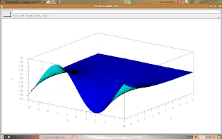
Now, I think it's interesting to upgrade our example.
Look the script:
-->t = 1:20;
-->x = meshgrid(t);
-->y = meshgrid(t($:-1:1))';
-->w = %pi/5;
-->s = sin(w*x);
-->plot(x, s + y, 'b.-');
-->plot(x', (s + y)', 'b.-');
The result:
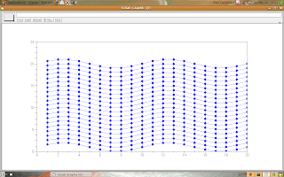
Try to change the grid and look what happens.
Wednesday, May 20, 2009
Simple graphs - 6
This is the last post about the simple uses of the plot(.) function.
In this post, we will learn how to mark the points on the line's graphs, like the following figure.
 The possible styles of markers in Scilab are:
Let's do some examples:
-->x1 = rand(10, 1);
-->plot(x1, 'x');
-->plot(x1, 'o');
-->t = 1:10;
-->x2 = exp(-0.1*t);
-->scf(); plot(t, x2, 'sr--');
-->scf(); plot(x1, x2, '^-.g');
The result:
Ok, now we are ready for start real applications.
In this post, we will learn how to mark the points on the line's graphs, like the following figure.
 The possible styles of markers in Scilab are:
- Plus sign;
- Circle;
- Asterisk;
- Point;
- Cross;
- Square;
- Diamond;
- Upward-pointing triangle;
- Downward-pointing triangle;
- Rightward-pointing triangle;
- Leftward-pointing triangle;
- Five-pointed star (pentagram);
- No marker (default).
Let's do some examples:
-->x1 = rand(10, 1);
-->plot(x1, 'x');
-->plot(x1, 'o');
-->t = 1:10;
-->x2 = exp(-0.1*t);
-->scf(); plot(t, x2, 'sr--');
-->scf(); plot(x1, x2, '^-.g');
The result:

Ok, now we are ready for start real applications.
Friday, May 15, 2009
Simple graphs - 5
Following our studies about the plot(.) function.
Now, let's learn how to change the line's style.
The possible line's styles in Scilab are:
Some examples:
-->x = 1:10;
-->y1 = x.^2 + 1;
-->plot(x, y1, "-");
-->y2 = x.^2 + 2;
-->plot(x + 10, y2, "--");
-->y3 = x.^2 + 3;
-->plot(x + 20, y3, ":");
-->y4 = x.^2 + 4;
-->plot(x + 30, y4, "-.");
The result:
You may use the line's styles with colors, for example:
--> plot(x, y, "r--");
Now, let's learn how to change the line's style.
The possible line's styles in Scilab are:
- Solid line (default);
- Dashed line;
- Dotted line;
- Dash-dotted line;
- No line.
Some examples:
-->x = 1:10;
-->y1 = x.^2 + 1;
-->plot(x, y1, "-");
-->y2 = x.^2 + 2;
-->plot(x + 10, y2, "--");
-->y3 = x.^2 + 3;
-->plot(x + 20, y3, ":");
-->y4 = x.^2 + 4;
-->plot(x + 30, y4, "-.");
The result:

You may use the line's styles with colors, for example:
--> plot(x, y, "r--");
Saturday, April 25, 2009
Simple graphs - 4
Let's continue our study about the plot(.) function.
Now, how change the graph's color?
The plot(.) has a argument that's a string.
We can do:
The possible colors are:
Let's do an example:
-->x = [-100:100]';
-->y1 = abs(x.^3)/1e+5;
-->y2 = x.^3 + x.^2 + 1;
-->y3 = tanh(0.01*x);
-->y2 = y2/max(y2);
-->plot(x, y1);
-->plot(x, y2, "r");
-->plot(x, y3, "g");
-->scf(); plot(x, y2, "k"); plot(x, y3, "y");
This example uses some functions that I had written about, so review the blog if you don't understand anything, or comment here.
The result is following.
Look that the default color is blue.
Now, how change the graph's color?
The plot(.) has a argument that's a string.
We can do:
- plot(x, y, color);
- plot(y, color);
The possible colors are:
- red ("r");
- green ("g");
- blue ("b");
- cyan ("c");
- magenta ("m");
- yellow ("y");
- black ("k");
- white ("w").
Let's do an example:
-->x = [-100:100]';
-->y1 = abs(x.^3)/1e+5;
-->y2 = x.^3 + x.^2 + 1;
-->y3 = tanh(0.01*x);
-->y2 = y2/max(y2);
-->plot(x, y1);
-->plot(x, y2, "r");
-->plot(x, y3, "g");
-->scf(); plot(x, y2, "k"); plot(x, y3, "y");
This example uses some functions that I had written about, so review the blog if you don't understand anything, or comment here.
The result is following.

Look that the default color is blue.
Saturday, April 18, 2009
Simple graphs - 3
I ask excuse me because I was doing other things, like a paper, and I could not post since 4, April.
Now, I finished the paper, and other things.
Let's continue talking about the plot(.) function.
The command for create a new window is scf(), it creates a blank window.
If you have a used window but you want to clear it, so you use the command clf();
Those commands (scf() and clf()) have no arguments.
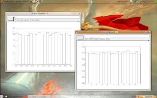
The scf() is utile for show many graphs simultaneously, like the following example.
The script is following, too:
-->x = 1:100;
-->w1 = %pi/3;
-->y1 = cos(w1*x);
-->w2 = %pi/7;
-->y2 = cos(w2*x);
-->plot(x, y1);
-->scf(); plot(x, y2);
The next posts will present how to change the colors and styles of the graphs, and how to put labels on the graphs.
Now, I finished the paper, and other things.
Let's continue talking about the plot(.) function.
The command for create a new window is scf(), it creates a blank window.
If you have a used window but you want to clear it, so you use the command clf();
Those commands (scf() and clf()) have no arguments.
The scf() is utile for show many graphs simultaneously, like the following example.
The script is following, too:
-->x = 1:100;
-->w1 = %pi/3;
-->y1 = cos(w1*x);
-->w2 = %pi/7;
-->y2 = cos(w2*x);
-->plot(x, y1);
-->scf(); plot(x, y2);

The next posts will present how to change the colors and styles of the graphs, and how to put labels on the graphs.
Friday, April 3, 2009
Simple graphs - 2
In the last post I introduced the plot(.) function.
That function is the simplest one for create graphs.
Let's learn something more about that function.
Try the commands:
-->x = rand(10, 1)
x =
0.2113249
0.7560439
0.0002211
0.3303271
0.6653811
0.6283918
0.8497452
0.6857310
0.8782165
0.0683740
-->plot(x);
The result is the following picture.
 Look the indexes (x axis), it starts on 1 and finishes on 10, because we did not put the x axis in the plot(.).
An other case:
-->y = rand(10, 1)
y =
0.3076091
0.9329616
0.2146008
0.312642
0.3616361
0.2922267
0.5664249
0.4826472
0.3321719
0.5935095
-->x = [0 1 2 3 4 5 6 7 8 9]'
x =
0.
1.
2.
3.
4.
5.
6.
7.
8.
9.
-->plot(x, y);
Now, the x axis starts on 0 and finishes on 9, because I put the coordinates of x axis.
That function is the simplest one for create graphs.
Let's learn something more about that function.
Try the commands:
-->x = rand(10, 1)
x =
0.2113249
0.7560439
0.0002211
0.3303271
0.6653811
0.6283918
0.8497452
0.6857310
0.8782165
0.0683740
-->plot(x);
The result is the following picture.
 Look the indexes (x axis), it starts on 1 and finishes on 10, because we did not put the x axis in the plot(.).
An other case:
-->y = rand(10, 1)
y =
0.3076091
0.9329616
0.2146008
0.312642
0.3616361
0.2922267
0.5664249
0.4826472
0.3321719
0.5935095
-->x = [0 1 2 3 4 5 6 7 8 9]'
x =
0.
1.
2.
3.
4.
5.
6.
7.
8.
9.
-->plot(x, y);

Now, the x axis starts on 0 and finishes on 9, because I put the coordinates of x axis.
Monday, March 30, 2009
Simple graphs - 1
This post is about the simplest graphs in Scilab.
Why do we need to do graphs? I think that's a unnecessary question.
The Scilab holds the last graph that we do.
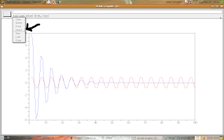
For example, if we need to do two graphs in a same screen, like the following figure.
Then we need to do the commands:
-->t = 1:100;
-->x1 = sin(t*%pi/3);
-->x2 = 10*exp(-0.1*t).*sin(t*%pi/3);
-->plot(x1, 'r');
-->plot(x2);
The showed graph needs to be saved, so we can click the option export (following figure), after we choose the format and the file's name.
All ready, the file is saved as a picture!
Why do we need to do graphs? I think that's a unnecessary question.
The Scilab holds the last graph that we do.
For example, if we need to do two graphs in a same screen, like the following figure.

Then we need to do the commands:
-->t = 1:100;
-->x1 = sin(t*%pi/3);
-->x2 = 10*exp(-0.1*t).*sin(t*%pi/3);
-->plot(x1, 'r');
-->plot(x2);
The showed graph needs to be saved, so we can click the option export (following figure), after we choose the format and the file's name.

All ready, the file is saved as a picture!
Thursday, March 19, 2009
Using files
Scilab has some functions for file manipulating.
Scilab can work with ASCII or binary files.
Why do we need to know how to use files?
If you want to share results, then give files of results is better than give scripts for generate them.
Okay, I think the most one knows what a file is.
Let's read the help (click the option like the picture).
Write "file manage" and select the first option: file.
This function is like the C function fopen().
The help contains some information over the function.
We can search for others functions, for example:
The most important functions are:
The functions read and write are used principally with matrices and vectors.
Look the examples:
-->x = rand(5,5)
x =
0.2113249 0.6283918 0.5608486 0.2320748 0.3076091
0.7560439 0.8497452 0.6623569 0.2312237 0.9329616
0.0002211 0.6857310 0.7263507 0.2164633 0.2146008
0.3303271 0.8782165 0.1985144 0.8833888 0.312642
0.6653811 0.0683740 0.5442573 0.6525135 0.3616361
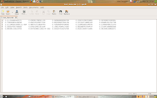
-->write("test_data.dat", x);
-->y1 = read("test_data.dat", 1, 2) // 1 line and 2 columns
y1 =
0.2113249 0.6283918
-->y2 = read("test_data.dat", 2, 2) // 2 lines and 2 columns
y2 =
0.2113249 0.6283918
0.7560439 0.8497452
-->y3 = read("test_data.dat", -1, 1) // -1 indicates that "all rows"
y3 =
0.2113249
0.7560439
0.0002211
0.3303271
0.6653811
-->>y4 = read("test_data.dat", -1, 5) // it reads the full file
y4 =
0.2113249 0.6283918 0.5608486 0.2320748 0.3076091
0.7560439 0.8497452 0.6623569 0.2312237 0.9329616
0.0002211 0.6857310 0.7263507 0.2164633 0.2146008
0.3303271 0.8782165 0.1985144 0.8833888 0.312642
0.6653811 0.0683740 0.5442573 0.6525135 0.3616361
The file "test_data.dat" (click on the picture for see the real size):
Scilab can work with ASCII or binary files.
Why do we need to know how to use files?
If you want to share results, then give files of results is better than give scripts for generate them.
Okay, I think the most one knows what a file is.
Let's read the help (click the option like the picture).

Write "file manage" and select the first option: file.
This function is like the C function fopen().
The help contains some information over the function.
We can search for others functions, for example:
- save;
- load;
- mopen;
- mclose;
- writeb;
- readb.
The most important functions are:
- read;
- write.
The functions read and write are used principally with matrices and vectors.
Look the examples:
-->x = rand(5,5)
x =
0.2113249 0.6283918 0.5608486 0.2320748 0.3076091
0.7560439 0.8497452 0.6623569 0.2312237 0.9329616
0.0002211 0.6857310 0.7263507 0.2164633 0.2146008
0.3303271 0.8782165 0.1985144 0.8833888 0.312642
0.6653811 0.0683740 0.5442573 0.6525135 0.3616361
-->write("test_data.dat", x);
-->y1 = read("test_data.dat", 1, 2) // 1 line and 2 columns
y1 =
0.2113249 0.6283918
-->y2 = read("test_data.dat", 2, 2) // 2 lines and 2 columns
y2 =
0.2113249 0.6283918
0.7560439 0.8497452
-->y3 = read("test_data.dat", -1, 1) // -1 indicates that "all rows"
y3 =
0.2113249
0.7560439
0.0002211
0.3303271
0.6653811
-->>y4 = read("test_data.dat", -1, 5) // it reads the full file
y4 =
0.2113249 0.6283918 0.5608486 0.2320748 0.3076091
0.7560439 0.8497452 0.6623569 0.2312237 0.9329616
0.0002211 0.6857310 0.7263507 0.2164633 0.2146008
0.3303271 0.8782165 0.1985144 0.8833888 0.312642
0.6653811 0.0683740 0.5442573 0.6525135 0.3616361
The file "test_data.dat" (click on the picture for see the real size):

Wednesday, March 11, 2009
Operations element by element
I was wrong, this post will talk about matrices and vectors (yet).
Let's talk about operations element by element.
For example, we have two matrices of same size and we need to multiply and to divide each element:
X = [x11 x12 x13;
x21 x22 x23;
x31 x32 x33].
Y = [y11 y12 y13;
y21 y22 y23;
y31 y32 y33].
Z1 = [x11*y11 x12*y12 x13*y13;
x21*y21 x22*y22 x23*y23;
x31*y31 x32*y32 x33*y33].
Z2 = [x11/y11 x12/y12 x13/y13;
x21/y21 x22/y22 x23/y23;
x31/y31 x32/y32 x33/y33].
The math doesn't have a operation for it, but it's possible using Scilab.
-->X = zeros(3,3);
-->X(:) = [1:9]'
X =
1. 4. 7.
2. 5. 8.
3. 6. 9.
-->Y = ones(3,3) + X'
Y =
2. 3. 4.
5. 6. 7.
8. 9. 10.
-->Z1 = X.*Y
Z1 =
2. 12. 28.
10. 30. 56.
24. 54. 90.
-->Z1 = X./Y
Z1 =
0.5 1.3333333 1.75
0.4 0.8333333 1.1428571
0.375 0.6666667 0.9
The operations sum and subtraction work element by element, like in matrices sum and subtraction.
If we need to use logic operations then we can use the operators:
-->X = rand(3,3) > 0.2
X =
F T T
T F T
T T T
-->Y = rand(3,3,'normal') > 0.5
Y =
T T F
T F T
F F F
-->Z1 = X & Y
Z1 =
F T F
T F T
F F F
-->Z2 = X | Y
Z2 =
T T T
T F T
T T T
-->Z3 = ~X
Z3 =
T F F
F T F
F F F
-->Z4 = (~X) | Y
Z4 =
T T F
T T T
F F F
That's all, I'm thinking about the next subject that I'll talk here. I accept suggestions.
Let's talk about operations element by element.
For example, we have two matrices of same size and we need to multiply and to divide each element:
X = [x11 x12 x13;
x21 x22 x23;
x31 x32 x33].
Y = [y11 y12 y13;
y21 y22 y23;
y31 y32 y33].
Z1 = [x11*y11 x12*y12 x13*y13;
x21*y21 x22*y22 x23*y23;
x31*y31 x32*y32 x33*y33].
Z2 = [x11/y11 x12/y12 x13/y13;
x21/y21 x22/y22 x23/y23;
x31/y31 x32/y32 x33/y33].
The math doesn't have a operation for it, but it's possible using Scilab.
-->X = zeros(3,3);
-->X(:) = [1:9]'
X =
1. 4. 7.
2. 5. 8.
3. 6. 9.
-->Y = ones(3,3) + X'
Y =
2. 3. 4.
5. 6. 7.
8. 9. 10.
-->Z1 = X.*Y
Z1 =
2. 12. 28.
10. 30. 56.
24. 54. 90.
-->Z1 = X./Y
Z1 =
0.5 1.3333333 1.75
0.4 0.8333333 1.1428571
0.375 0.6666667 0.9
The operations sum and subtraction work element by element, like in matrices sum and subtraction.
Logic operations
If we need to use logic operations then we can use the operators:
- & - AND;
- | - OR;
- ~ - NOT.
-->X = rand(3,3) > 0.2
X =
F T T
T F T
T T T
-->Y = rand(3,3,'normal') > 0.5
Y =
T T F
T F T
F F F
-->Z1 = X & Y
Z1 =
F T F
T F T
F F F
-->Z2 = X | Y
Z2 =
T T T
T F T
T T T
-->Z3 = ~X
Z3 =
T F F
F T F
F F F
-->Z4 = (~X) | Y
Z4 =
T T F
T T T
F F F
That's all, I'm thinking about the next subject that I'll talk here. I accept suggestions.
Tuesday, March 3, 2009
Vectors and Matrices - 4
I think this is the last basic post about vectors and matrices.
Let's do logic operations with vectors and matrices.
Our example uses more common informations.
We have a vector and each element is the height of a person (in meters).
Now, we need to know who is taller than 1.80m.
So, we can do an analysis element by element, like this:
v(1) > 1.80
v(2) > 1.80
v(3) > 1.80
v(4) > 1.80
v(5) > 1.80
v(6) > 1.80
v(7) > 1.80
But, the Scilab has a very simple solution.
v > 1.8 // this operation is non-dependent of vector's dimensionality
Look the script.
-->v = [1.55 1.82 1.48 1.71 1.62 1.94 2.00]'
v =
1.55
1.82
1.48
1.71
1.62
1.94
2.
-->v > 1.8
ans =
F
T
F
F
F
T
T
But, if we want the positions of the elements (people) taller than 1.80m then we can do this:
-->positions = find(v > 1.8)
positions =
2. 6. 7.
The elements in v these are taller than 1.8m are the 2nd (1.82m), 6th (1.94m) and 7th (2.00m).
We can do the same analysis for matrices.
A very useful example is a binary matrix with equal probability of zeros and ones.
Look the script and post to me your comments.
-->x = rand(3, 3)
x =
0.5667211 0.0568928 0.7279222
0.5711639 0.5595937 0.2677766
0.8160110 0.1249340 0.5465335
-->y = x > 0.5
y =
T F T
T T F
T F T
In showed example we have more ones ("Trues"), I ask: why?
Let's do logic operations with vectors and matrices.
Our example uses more common informations.
We have a vector and each element is the height of a person (in meters).
v = [1.55 1.82 1.48 1.71 1.62 1.94 2.00]'
Now, we need to know who is taller than 1.80m.
So, we can do an analysis element by element, like this:
v(1) > 1.80
v(2) > 1.80
v(3) > 1.80
v(4) > 1.80
v(5) > 1.80
v(6) > 1.80
v(7) > 1.80
But, the Scilab has a very simple solution.
v > 1.8 // this operation is non-dependent of vector's dimensionality
Look the script.
-->v = [1.55 1.82 1.48 1.71 1.62 1.94 2.00]'
v =
1.55
1.82
1.48
1.71
1.62
1.94
2.
-->v > 1.8
ans =
F
T
F
F
F
T
T
But, if we want the positions of the elements (people) taller than 1.80m then we can do this:
-->positions = find(v > 1.8)
positions =
2. 6. 7.
The elements in v these are taller than 1.8m are the 2nd (1.82m), 6th (1.94m) and 7th (2.00m).
We can do the same analysis for matrices.
A very useful example is a binary matrix with equal probability of zeros and ones.
Look the script and post to me your comments.
-->x = rand(3, 3)
x =
0.5667211 0.0568928 0.7279222
0.5711639 0.5595937 0.2677766
0.8160110 0.1249340 0.5465335
-->y = x > 0.5
y =
T F T
T T F
T F T
In showed example we have more ones ("Trues"), I ask: why?
Friday, February 27, 2009
Logic Operations
I think the most one knows something about logic operations, but let's do a little review.
Logic operations are used for analysis of situations like:
The logic operations combine two or more situations, for example:
I'm 22, my father's 52 and my sister's 19.
The question: who is the older?
The solution:
The logic operators are used with logic variables. Logic variables are like numeric variables but the values are true or false.
The basic logic operators are: {not, or, and}
The not is a unary operator and the others are binary operators.
So, follow the possible logic situations for each operation:
NOT
AND
OR
A mental train.
If I want a racket and a ball but I have just a racket I'm not satisfied. But, If I want a ball of basketball or a ball of soccer, so I need one ball or both.
The Scilab has that three operators.
The operator '~' is the not.
The operator '|' is the or.
The operator '&' is the and.
The operations or and and can be applied on vectors with the functions or(.) and and(.).
Let's play now.
-->x = 10;
-->y = 15;
-->z = x + y
z =
25.
-->(x > y) & (z > x) // x is smaller than y then the first operation is false
ans =
F
-->(x > y) | (z > x) // z is bigger than x then the second operation is true
ans =
T
-->~((x > y) & (z > x)) // the result is the inverse of the first result
ans =
T
-->~((x > y) | (z > x)) // the result is the inverse of the second result
ans =
F
The results are F (false) or T (true) because logic operations give logic results.
If you want use the variables with logic values:
-->r1 = %F
r1 =
F
-->r2 = %T
r2 =
T
-->and([r1 r2])
ans =
F
-->or([r1 r2])
ans =
T
For finish the post, if you use a numeric variable with logic operators, thus the Scilab interprets the 0 (zero) as false and different of 0 (zero) as true.
-->x = 0;
-->y = 2;
-->z = -5;
-->x | y | z
ans =
T
-->x & y & z
ans =
F
-->x & z
ans =
F
-->x & y
ans =
F
-->y & z
ans =
T
Logic operations are used for analysis of situations like:
- 2 is bigger than 3? - false
- the vector [1 2 3 4] is larger than [1 3 5]? - true
- the word 'horse' is smaller than 'dog'? - false
The logic operations combine two or more situations, for example:
I'm 22, my father's 52 and my sister's 19.
The question: who is the older?
The solution:
- if I'm older than my father and my sister then I'm the older.
- if my father's older than me and my sister then he's the older.
- if my sister's older than my father and me then she's the older.
The logic operators are used with logic variables. Logic variables are like numeric variables but the values are true or false.
The basic logic operators are: {not, or, and}
The not is a unary operator and the others are binary operators.
So, follow the possible logic situations for each operation:
NOT
- not(true) is false
- not(false) is true
AND
- false and false is false
- false and true is false
- true and false is false
- true and true is true
OR
- false or false is false
- false or true is true
- true or false is true
- true or true is true
A mental train.
If I want a racket and a ball but I have just a racket I'm not satisfied. But, If I want a ball of basketball or a ball of soccer, so I need one ball or both.
The Scilab has that three operators.
The operator '~' is the not.
The operator '|' is the or.
The operator '&' is the and.
The operations or and and can be applied on vectors with the functions or(.) and and(.).
Let's play now.
-->x = 10;
-->y = 15;
-->z = x + y
z =
25.
-->(x > y) & (z > x) // x is smaller than y then the first operation is false
ans =
F
-->(x > y) | (z > x) // z is bigger than x then the second operation is true
ans =
T
-->~((x > y) & (z > x)) // the result is the inverse of the first result
ans =
T
-->~((x > y) | (z > x)) // the result is the inverse of the second result
ans =
F
The results are F (false) or T (true) because logic operations give logic results.
If you want use the variables with logic values:
-->r1 = %F
r1 =
F
-->r2 = %T
r2 =
T
-->and([r1 r2])
ans =
F
-->or([r1 r2])
ans =
T
For finish the post, if you use a numeric variable with logic operators, thus the Scilab interprets the 0 (zero) as false and different of 0 (zero) as true.
-->x = 0;
-->y = 2;
-->z = -5;
-->x | y | z
ans =
T
-->x & y & z
ans =
F
-->x & z
ans =
F
-->x & y
ans =
F
-->y & z
ans =
T
Wednesday, February 11, 2009
Vectors and Matrices - 3
Now, I'll write about specific functions for matrices.
The most common functions that I use:
Let's play, with them.
-->eye(3,3) // identity matrix 3 lines and 3 columns*
ans =
1. 0. 0.
0. 1. 0.
0. 0. 1.
-->rand(5,2) // matrix (5 lines and 2 columns) of random numbers with uniform probability distribution between [0,1]
ans =
0.0683740 0.5442573
0.5608486 0.2320748
0.6623569 0.2312237
0.7263507 0.2164633
0.1985144 0.8833888
-->rand(2,5,'normal') // matrix (2 lines and 5 columns) of random numbers with normal (Gaussian) distribution (mean = 0 and variance = 1)
ans =
1.0478272 - 1.4061926 - 1.7350313 - 0.2143931 2.5891773
- 1.3218008 - 1.0384734 0.5546874 - 2.0735088 0.0424792
-->det(eye(4,4)) // determinant of identity matrix 4 x 4
ans =
1.
-->X = rand(5,5) // X is a matrix (5 x 5) with random values between [0,1]
X =
0.4368588 0.0437334 0.1280058 0.1531217 0.8784126
0.2693125 0.4818509 0.7783129 0.6970851 0.1138360
0.6325745 0.2639556 0.2119030 0.8415518 0.1998338
0.4051954 0.4148104 0.1121355 0.4062025 0.5618661
0.9184708 0.2806498 0.6856896 0.4094825 0.5896177
-->det_X = det(X) // det_X is the determinant of X
det_X =
- 0.0799884
-->[py px] = find(eye(3,3)) // px is the positions (x-coordinates) of numbers nonzeros and py is the positions (y-coordinates) of numbers nonzeros
px =
1. 2. 3.
py =
1. 2. 3.
-->[py px] = find(~eye(3,3)) // the ~ is the logic negative operation, so (~0) = 1 and (~1) = 0**
px =
1. 1. 2. 2. 3. 3.
py =
2. 3. 1. 3. 1. 2.
-->X // the variable X (X = rand(5,5))
X =
0.4368588 0.0437334 0.1280058 0.1531217 0.8784126
0.2693125 0.4818509 0.7783129 0.6970851 0.1138360
0.6325745 0.2639556 0.2119030 0.8415518 0.1998338
0.4051954 0.4148104 0.1121355 0.4062025 0.5618661
0.9184708 0.2806498 0.6856896 0.4094825 0.5896177
-->sum(X,'r') // sum over the columns of X (row of values)
ans =
2.6624119 1.4850001 1.9160468 2.5074436 2.3435661
-->sum(X,'c') // sum over the lines of X (column of values)
ans =
1.6401323
2.3403973
2.1498187
1.9002098
2.8839105
-->sum(X) // sum of all elements of X
ans =
10.914469
So, if anyone has any question, then everyone can do comments.
----------
* If you do a command without send the return to a variable, then the Scilab creates the variable ans (answer) with the return or function or operation.
For example:
-->1+1
ans =
2.
-->cos(%pi)
ans =
- 1.
-->sin(%pi/2)+1
ans =
2.
** I'll write about logic operations in next posts.
The most common functions that I use:
- eye(m,n) - identity matrix;
- zeros(m,n) - matrix of zeros;
- ones(m,n) - matrix of ones;
- det(X) - determinant;
- inv(X) - matrix inverse;
- pinv(A,[tol]) - pseudoinverse;
- sum(x,[key]) - sum (row sum, column sum) of vector/matrix entries;
- prod(x,[key]) - product (row sum, column sum) of vector/matrix entries;
- mean(x,[key]) - mean (row sum, column sum) of vector/matrix entries;
- stdev(x,[key]) - standard deviation (row sum, column sum) of vector/matrix entries;
- geomean(x,[key]) - geometric mean (row sum, column sum) of vector/matrix entries;
- harmean(x,[key]) - harmonic mean (row sum, column sum) of vector/matrix entries;
- msd(x,[key]) - mean squared deviation (row sum, column sum) of vector/matrix entries;
- rand(m1,m2,.. [,key]) - random number generator;
- grand(m, n, dist_type [,p1,...,pk]) - Random number generator(s);
- find(X) - find indices of boolean vector or matrix true elements.
Let's play, with them.
-->eye(3,3) // identity matrix 3 lines and 3 columns*
ans =
1. 0. 0.
0. 1. 0.
0. 0. 1.
-->rand(5,2) // matrix (5 lines and 2 columns) of random numbers with uniform probability distribution between [0,1]
ans =
0.0683740 0.5442573
0.5608486 0.2320748
0.6623569 0.2312237
0.7263507 0.2164633
0.1985144 0.8833888
-->rand(2,5,'normal') // matrix (2 lines and 5 columns) of random numbers with normal (Gaussian) distribution (mean = 0 and variance = 1)
ans =
1.0478272 - 1.4061926 - 1.7350313 - 0.2143931 2.5891773
- 1.3218008 - 1.0384734 0.5546874 - 2.0735088 0.0424792
-->det(eye(4,4)) // determinant of identity matrix 4 x 4
ans =
1.
-->X = rand(5,5) // X is a matrix (5 x 5) with random values between [0,1]
X =
0.4368588 0.0437334 0.1280058 0.1531217 0.8784126
0.2693125 0.4818509 0.7783129 0.6970851 0.1138360
0.6325745 0.2639556 0.2119030 0.8415518 0.1998338
0.4051954 0.4148104 0.1121355 0.4062025 0.5618661
0.9184708 0.2806498 0.6856896 0.4094825 0.5896177
-->det_X = det(X) // det_X is the determinant of X
det_X =
- 0.0799884
-->[py px] = find(eye(3,3)) // px is the positions (x-coordinates) of numbers nonzeros and py is the positions (y-coordinates) of numbers nonzeros
px =
1. 2. 3.
py =
1. 2. 3.
-->[py px] = find(~eye(3,3)) // the ~ is the logic negative operation, so (~0) = 1 and (~1) = 0**
px =
1. 1. 2. 2. 3. 3.
py =
2. 3. 1. 3. 1. 2.
-->X // the variable X (X = rand(5,5))
X =
0.4368588 0.0437334 0.1280058 0.1531217 0.8784126
0.2693125 0.4818509 0.7783129 0.6970851 0.1138360
0.6325745 0.2639556 0.2119030 0.8415518 0.1998338
0.4051954 0.4148104 0.1121355 0.4062025 0.5618661
0.9184708 0.2806498 0.6856896 0.4094825 0.5896177
-->sum(X,'r') // sum over the columns of X (row of values)
ans =
2.6624119 1.4850001 1.9160468 2.5074436 2.3435661
-->sum(X,'c') // sum over the lines of X (column of values)
ans =
1.6401323
2.3403973
2.1498187
1.9002098
2.8839105
-->sum(X) // sum of all elements of X
ans =
10.914469
So, if anyone has any question, then everyone can do comments.
----------
* If you do a command without send the return to a variable, then the Scilab creates the variable ans (answer) with the return or function or operation.
For example:
-->1+1
ans =
2.
-->cos(%pi)
ans =
- 1.
-->sin(%pi/2)+1
ans =
2.
** I'll write about logic operations in next posts.
Saturday, February 7, 2009
Vectors and Matrices - 2
In the last post, I wrote about simple operations with matrices. Now, I want to talk about the functions and we will use them on matrices and vectors.
All right, let's start. The Scilab has many math functions, like sin, cos, tan, asin, acos, atan, exp, log, etc....
All functions can be used on any type of numeric variable (scalar, vector, matrix or tensor).
First example:
-->x = [1 0 1;
-->0 1 0;
-->1 0 1]
x =
1. 0. 1.
0. 1. 0.
1. 0. 1.
-->y = cos(%pi*x) // the Scilab has some common values, I know PI (%pi = 3.1415927) and E (%e = 2.7182818)
y =
- 1. 1. - 1.
1. - 1. 1.
- 1. 1. - 1.
Look that cos(%pi) = -1 and cos(0) = 1 (remember the trigonometric circle).
So, operations with matrices create new matrices, and the new matrices can be used on the new operations or functions.
Let's go to the second example.
-->x = [1 2 3]
x =
1. 2. 3.
-->y = [3;
-->2;
-->1]
y =
3.
2.
1.
-->z1 = exp(x*y)
z1 =
22026.466
-->z2 = exp(y*x)
z2 =
20.085537 403.42879 8103.0839
7.3890561 54.59815 403.42879
2.7182818 7.3890561 20.085537
The operation x*y results in
x*y = [1*3 + 2*2 + 3*1] = [3 + 4 + 3] = 10.
The operation y*x results in
y*x =
[3*1 3*2 3*3;
2*1 2*2 2*3;
1*1 1*2 1*3] =
[3 6 9;
2 4 6;
1 2 3].
The function exp(.) returns the natural exponential (exp(x) = %e^x).
Ok, let's finish here. Who wants more, do comments.
Saturday, January 31, 2009
Vectors and Matrices - 1
The Scilab is like Matlab (Matrix Lab), I don't like Matlab but it's other thing.
The Scilab was created for matrix manipulation, so it can operate matrices (and similars) naturally.
This is the first post about vectors and matrices.
Let's do something.
Get a vector
x = [1 2 3 4]' (x is a column vector)
and a matrix
A = [1 2 3 4;
1 2 3 4;
1 2 3 4;
1 2 3 4].
If y = A x (matrix multiplication), then y = [x[1]A[1,1]+x[2]A[2,1]+x[3]A[3,1]+x[4]A[4,1] x[1]A[1,2]+x[2]A[2,2]+x[3]A[3,2]+x[4]A[4,2] x[1]A[1,3]+x[2]A[2,3]+x[3]A[3,3]+x[4]A[4,3] x[1]A[1,4]+x[2]A[2,4]+x[3]A[3,4]+x[4]A[4,4]] = [1²+2²+3²+4² 1²+2²+3²+4² 1²+2²+3²+4² 1²+2²+3²+4²] = [30 30 30 30].
For who studies linear algebra, the equation y = A x is a generic linear system of 1st order.
Using Scilab, we can do the commands.
-->x = [1 2 3 4]'; // the apostrophe { ' } indicates the transposition, so x is a column vector because [1 2 3 4] is a line vector and x is [1 2 3 4] transpose.
-->A = [1 2 3 4;
-->1 2 3 4;
-->1 2 3 4;
-->1 2 3 4];
-->y = A*x
y =
30.
30.
30.
30.
Look that y is a column vector like x (with 4 lines), it's correct because A is a square matrix (with 4 lines and 4 columns) and x is a column vector (with 4 lines).
Using the rule dim(y) = dim(Ax) = [number of lines of A, (number of columns of A, number of lines of x), number of columns of x] = [number of lines of A, number of columns of x] (parenthesis out).
I'll do more posts about vectors and matrices. Wait and see.
Subscribe to:
Posts (Atom)