Monday, March 30, 2009

Simple graphs - 1

This post is about the simplest graphs in Scilab.

Why do we need to do graphs? I think that's a unnecessary question.

The Scilab holds the last graph that we do.

For example, if we need to do two graphs in a same screen, like the following figure.


Then we need to do the commands:

-->t = 1:100;

-->x1 = sin(t*%pi/3);

-->x2 = 10*exp(-0.1*t).*sin(t*%pi/3);

-->plot(x1, 'r');

-->plot(x2);

The showed graph needs to be saved, so we can click the option export (following figure), after we choose the format and the file's name.


All ready, the file is saved as a picture!

Thursday, March 19, 2009

Using files

Scilab has some functions for file manipulating.

Scilab can work with ASCII or binary files.

Why do we need to know how to use files?

If you want to share results, then give files of results is better than give scripts for generate them.

Okay, I think the most one knows what a file is.

Let's read the help (click the option like the picture).


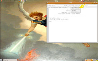
Write "file manage" and select the first option: file.

This function is like the C function fopen().

The help contains some information over the function.

We can search for others functions, for example:

  • save;
  • load;
  • mopen;
  • mclose;
  • writeb;
  • readb.
But, I don't think these functions very necessary now, maybe in an other situation.

The most important functions are:

  • read;
  • write.
We create files using write and load files using read.

The functions read and write are used principally with matrices and vectors.

Look the examples:

-->x = rand(5,5)
x =

0.2113249 0.6283918 0.5608486 0.2320748 0.3076091
0.7560439 0.8497452 0.6623569 0.2312237 0.9329616
0.0002211 0.6857310 0.7263507 0.2164633 0.2146008
0.3303271 0.8782165 0.1985144 0.8833888 0.312642
0.6653811 0.0683740 0.5442573 0.6525135 0.3616361

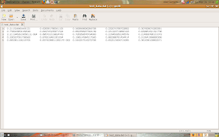
-->write("test_data.dat", x);

-->y1 = read("test_data.dat", 1, 2) // 1 line and 2 columns
y1 =

0.2113249 0.6283918

-->y2 = read("test_data.dat", 2, 2) // 2 lines and 2 columns
y2 =

0.2113249 0.6283918
0.7560439 0.8497452

-->y3 = read("test_data.dat", -1, 1) // -1 indicates that "all rows"
y3 =

0.2113249
0.7560439
0.0002211
0.3303271
0.6653811

-->>y4 = read("test_data.dat", -1, 5) // it reads the full file
y4 =

0.2113249 0.6283918 0.5608486 0.2320748 0.3076091
0.7560439 0.8497452 0.6623569 0.2312237 0.9329616
0.0002211 0.6857310 0.7263507 0.2164633 0.2146008
0.3303271 0.8782165 0.1985144 0.8833888 0.312642
0.6653811 0.0683740 0.5442573 0.6525135 0.3616361


The file "test_data.dat" (click on the picture for see the real size):

Wednesday, March 11, 2009

Operations element by element

I was wrong, this post will talk about matrices and vectors (yet).

Let's talk about operations element by element.

For example, we have two matrices of same size and we need to multiply and to divide each element:

X = [x11 x12 x13;
x21 x22 x23;
x31 x32 x33].

Y = [y11 y12 y13;
y21 y22 y23;
y31 y32 y33].

Z1 = [x11*y11 x12*y12 x13*y13;
x21*y21 x22*y22 x23*y23;
x31*y31 x32*y32 x33*y33].

Z2 = [x11/y11 x12/y12 x13/y13;
x21/y21 x22/y22 x23/y23;
x31/y31 x32/y32 x33/y33].

The math doesn't have a operation for it, but it's possible using Scilab.

-->X = zeros(3,3);

-->X(:) = [1:9]'
X =

1. 4. 7.
2. 5. 8.
3. 6. 9.

-->Y = ones(3,3) + X'
Y =

2. 3. 4.
5. 6. 7.
8. 9. 10.

-->Z1 = X.*Y
Z1 =

2. 12. 28.
10. 30. 56.
24. 54. 90.

-->Z1 = X./Y
Z1 =

0.5 1.3333333 1.75
0.4 0.8333333 1.1428571
0.375 0.6666667 0.9


The operations sum and subtraction work element by element, like in matrices sum and subtraction.


Logic operations

If we need to use logic operations then we can use the operators:

  • & - AND;
  • | - OR;
  • ~ - NOT.

-->X = rand(3,3) > 0.2
X =

F T T
T F T
T T T

-->Y = rand(3,3,'normal') > 0.5
Y =

T T F
T F T
F F F

-->Z1 = X & Y
Z1 =

F T F
T F T
F F F

-->Z2 = X | Y
Z2 =

T T T
T F T
T T T

-->Z3 = ~X
Z3 =

T F F
F T F
F F F

-->Z4 = (~X) | Y
Z4 =

T T F
T T T
F F F

That's all, I'm thinking about the next subject that I'll talk here. I accept suggestions.

Tuesday, March 3, 2009

Vectors and Matrices - 4

I think this is the last basic post about vectors and matrices.

Let's do logic operations with vectors and matrices.

Our example uses more common informations.

We have a vector and each element is the height of a person (in meters).

v = [1.55 1.82 1.48 1.71 1.62 1.94 2.00]'

Now, we need to know who is taller than 1.80m.

So, we can do an analysis element by element, like this:

v(1) > 1.80
v(2) > 1.80
v(3) > 1.80
v(4) > 1.80
v(5) > 1.80
v(6) > 1.80
v(7) > 1.80

But, the Scilab has a very simple solution.

v > 1.8 // this operation is non-dependent of vector's dimensionality

Look the script.

-->v = [1.55 1.82 1.48 1.71 1.62 1.94 2.00]'
v =

1.55
1.82
1.48
1.71
1.62
1.94
2.

-->v > 1.8
ans =

F
T
F
F
F
T
T

But, if we want the positions of the elements (people) taller than 1.80m then we can do this:

-->positions = find(v > 1.8)
positions =

2. 6. 7.


The elements in v these are taller than 1.8m are the 2nd (1.82m), 6th (1.94m) and 7th (2.00m).

We can do the same analysis for matrices.

A very useful example is a binary matrix with equal probability of zeros and ones.

Look the script and post to me your comments.

-->x = rand(3, 3)
x =

0.5667211 0.0568928 0.7279222
0.5711639 0.5595937 0.2677766
0.8160110 0.1249340 0.5465335

-->y = x > 0.5
y =

T F T
T T F
T F T

In showed example we have more ones ("Trues"), I ask: why?