I made a video with some examples.
Look that the Scilab presents the example's codes.
If the readers like my initiative, then I can make more videos.
Monday, June 29, 2009
Friday, June 26, 2009
Polynomials
Let's learn something different today.
We study polynomials at school, so we are going to learn anything about how Scilab works with them.
First, this post is moved to fractions of polynomials, for example*:
For work with polynomials in Scilab, we use the %s as the variable. Look the example**:
-->A = %s^2 + %s + 1
A =
2
1 + s + s
-->B = %s + 2
B =
2 + s
-->R = A*B
R =
2 3
2 + 3s + 3s + s
-->Q = A/B
Q =
2
1 + s + s
---------
2 + s
-->S = A + B
S =
2
3 + 2s + s
-->D = A - B
D =
2
- 1 + s
Observe that Scilab works correctly with the coefficients.
Now, let's work more, if we have a fraction of polynomials and we need just the denominator:
-->Q = (%s + 1)/(%s^2 + 2*%s + 2)
Q =
1 + s
---------
2
2 + 2s + s
-->Dem = denom(Q)
Dem =
2
2 + 2s + s
Following with the example, now we need just the numerator:
-->Num = numer(Q)
Num =
1 + s
And now, we need the roots of the denominator and of the numerator:
-->R_Dem = roots(Dem)
R_Dem =
- 1. + i
- 1. - i
-->R_Num = roots(Num)
R_Num =
- 1.
If anyone has studied linear systems, post a comment here.
If nobody has studied it, you can make a post too.
-----------------------
* I use OpenOffice Math for create the equations.
** The blog doesn't work with white spaces, but Scilab puts the higher coefficients after.
We study polynomials at school, so we are going to learn anything about how Scilab works with them.
First, this post is moved to fractions of polynomials, for example*:

For work with polynomials in Scilab, we use the %s as the variable. Look the example**:
-->A = %s^2 + %s + 1
A =
2
1 + s + s
-->B = %s + 2
B =
2 + s
-->R = A*B
R =
2 3
2 + 3s + 3s + s
-->Q = A/B
Q =
2
1 + s + s
---------
2 + s
-->S = A + B
S =
2
3 + 2s + s
-->D = A - B
D =
2
- 1 + s
Observe that Scilab works correctly with the coefficients.
Now, let's work more, if we have a fraction of polynomials and we need just the denominator:
-->Q = (%s + 1)/(%s^2 + 2*%s + 2)
Q =
1 + s
---------
2
2 + 2s + s
-->Dem = denom(Q)
Dem =
2
2 + 2s + s
Following with the example, now we need just the numerator:
-->Num = numer(Q)
Num =
1 + s
And now, we need the roots of the denominator and of the numerator:
-->R_Dem = roots(Dem)
R_Dem =
- 1. + i
- 1. - i
-->R_Num = roots(Num)
R_Num =
- 1.
If anyone has studied linear systems, post a comment here.
If nobody has studied it, you can make a post too.
-----------------------
* I use OpenOffice Math for create the equations.
** The blog doesn't work with white spaces, but Scilab puts the higher coefficients after.
Tuesday, June 23, 2009
Plot 3D - surface
Ok, the world is learning how to use Scilab. I like it a lot!
Now, let's make surfaces using the function plot3d(.).
This function is called like this: plot3d(x, y, z);
Where x and y are vectors and z is a matrix.
Look the example:
-->d = -3:3;
-->[x y] = meshgrid(d)
y =
- 3. - 3. - 3. - 3. - 3. - 3. - 3.
- 2. - 2. - 2. - 2. - 2. - 2. - 2.
- 1. - 1. - 1. - 1. - 1. - 1. - 1.
0. 0. 0. 0. 0. 0. 0.
1. 1. 1. 1. 1. 1. 1.
2. 2. 2. 2. 2. 2. 2.
3. 3. 3. 3. 3. 3. 3.
x =
- 3. - 2. - 1. 0. 1. 2. 3.
- 3. - 2. - 1. 0. 1. 2. 3.
- 3. - 2. - 1. 0. 1. 2. 3.
- 3. - 2. - 1. 0. 1. 2. 3.
- 3. - 2. - 1. 0. 1. 2. 3.
- 3. - 2. - 1. 0. 1. 2. 3.
- 3. - 2. - 1. 0. 1. 2. 3.
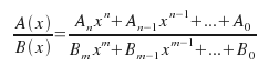
-->z = 9 - (x.^2 + y.^2);
-->plot3d(d, d, z);
The result is showed:
The coordinates x and y were the vector d (-3:3).
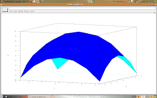
We can make any surface, so let's think in other surface. Look the next example:
-->x = -5:0.1:5;
-->y = 0:0.1:10;
-->[xc yc] = meshgrid(x, y);
-->w = %pi/4;
-->b = -0.5;
-->z = exp(b*yc).*sin(w*xc);
-->plot3d(x, y, z);
The result:
Try to make tests and generate surfaces.
Now, let's make surfaces using the function plot3d(.).
This function is called like this: plot3d(x, y, z);
Where x and y are vectors and z is a matrix.
Look the example:
-->d = -3:3;
-->[x y] = meshgrid(d)
y =
- 3. - 3. - 3. - 3. - 3. - 3. - 3.
- 2. - 2. - 2. - 2. - 2. - 2. - 2.
- 1. - 1. - 1. - 1. - 1. - 1. - 1.
0. 0. 0. 0. 0. 0. 0.
1. 1. 1. 1. 1. 1. 1.
2. 2. 2. 2. 2. 2. 2.
3. 3. 3. 3. 3. 3. 3.
x =
- 3. - 2. - 1. 0. 1. 2. 3.
- 3. - 2. - 1. 0. 1. 2. 3.
- 3. - 2. - 1. 0. 1. 2. 3.
- 3. - 2. - 1. 0. 1. 2. 3.
- 3. - 2. - 1. 0. 1. 2. 3.
- 3. - 2. - 1. 0. 1. 2. 3.
- 3. - 2. - 1. 0. 1. 2. 3.
-->z = 9 - (x.^2 + y.^2);
-->plot3d(d, d, z);
The result is showed:

The coordinates x and y were the vector d (-3:3).
We can make any surface, so let's think in other surface. Look the next example:
-->x = -5:0.1:5;
-->y = 0:0.1:10;
-->[xc yc] = meshgrid(x, y);
-->w = %pi/4;
-->b = -0.5;
-->z = exp(b*yc).*sin(w*xc);
-->plot3d(x, y, z);
The result:

Try to make tests and generate surfaces.
Friday, June 12, 2009
Plotting vectors like an animation
The last post received a comment, so I thought the readers could like to see anything more about how to plot vectors.
Let's use the Scilab's text editor, click the 'Editor' button and write the scripts, look the images.
 Opening the editor.
 Using the editor.
Read the buttons for use the editor's resources.
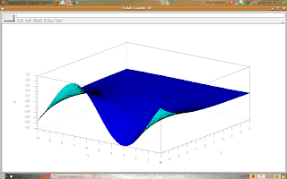
Now, let's see what happens when the following script is executed:
r = 0.1:0.1:10;
w = %pi/10;
x_i = 0;
y_i = 0;
for t = 1:length(r),
x_f = r(t)*cos(w*t);
y_f = r(t)*sin(w*t);
champ(x_i, y_i, x_f - x_i, y_f - y_i, 0.1);
x_i = x_f;
y_i = y_f;
sleep(100);
end;
--------------
The result:
Let's use the Scilab's text editor, click the 'Editor' button and write the scripts, look the images.
 Opening the editor.
 Using the editor.
Read the buttons for use the editor's resources.
Now, let's see what happens when the following script is executed:
r = 0.1:0.1:10;
w = %pi/10;
x_i = 0;
y_i = 0;
for t = 1:length(r),
x_f = r(t)*cos(w*t);
y_f = r(t)*sin(w*t);
champ(x_i, y_i, x_f - x_i, y_f - y_i, 0.1);
x_i = x_f;
y_i = y_f;
sleep(100);
end;
--------------
The result:
Friday, June 5, 2009
Plotting vectors
I received an e-mail from a reader, I feel happy with it, so if anyone needs help, I'm receiving asks.
So, let's follow with our Scilab's tutorial.
This post is about plotting vectors, like the picture.

This kind of plotting is very common for applications on electromagnetism or analysis of fluids.
In Scilab, we can use the champ(.) function for plotting vectors.
Look the following script:
-->x = -5:5;
-->y = 0:4;
-->[xv yv] = meshgrid(x, y)
yv =
0. 0. 0. 0. 0. 0. 0. 0. 0. 0. 0.
1. 1. 1. 1. 1. 1. 1. 1. 1. 1. 1.
2. 2. 2. 2. 2. 2. 2. 2. 2. 2. 2.
3. 3. 3. 3. 3. 3. 3. 3. 3. 3. 3.
4. 4. 4. 4. 4. 4. 4. 4. 4. 4. 4.
xv =
- 5. - 4. - 3. - 2. - 1. 0. 1. 2. 3. 4. 5.
- 5. - 4. - 3. - 2. - 1. 0. 1. 2. 3. 4. 5.
- 5. - 4. - 3. - 2. - 1. 0. 1. 2. 3. 4. 5.
- 5. - 4. - 3. - 2. - 1. 0. 1. 2. 3. 4. 5.
- 5. - 4. - 3. - 2. - 1. 0. 1. 2. 3. 4. 5.
-->wx = %pi/3;
-->xv = cos(wx*xv);
-->yv = yv/max(yv);
-->champ(x, y, xv', yv', 1);
The result is showed following:
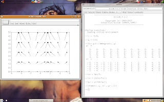
The champ(.) has five arguments, the first and the second are the coordinates of each vector, the third and the fourth are the components of each vector, and the fifth is a correction argument (for normalization).
Try to make graphs and say me what happens.
Subscribe to:
Posts (Atom)