Saturday, August 29, 2009

Discrete convolution properties - 1

I received a comment here. And, this post is about discrete convolution properties.

The continuous form of the convolution is given by:

So, the discrete form is given by:

If x[n] and h[n] are limited in the time ({x[n] = 0 if n <> Xn} and {h[n] = 0 if n <> Hn}), then the convolution is implemented as follow:

Let's suppose Xn > Hn (if Hn > Xn, the analysis is the same).

The equation is separated in three cases:

Case 1
Case 2
Case 3
Any other situation, y[n] = 0.

If you make an analysis in y[n], you'll see that y[n] = 0, if n <> Xn + Hn - 1.

Some other properties of the discrete convolution are the same than the continuous convolution:
  • x[n] * h[n] = h[n] * x[n];
  • x[n]*(h1[n]*h2[n]) = (x[n]*h1[n])*h2[n];
  • x[n]*(h1[n] + h2[n]) = x[n]*h1[n] + x[n]*h2[n];
  • a(x[n]*h[n]) = (ax[n])*h[n] = x[n]*(ah[n]), a is real;
  • x[n]*d[n] = x[n], d[n] = 1 if n = 0 and d[n] = 0 if n is not null;
  • x[n]*xi[n] = d[n], xi[n] is the inverse of x[n].
Ok, now you can make your own script for the convolution and try the properties.

Say me what happens.

Tuesday, August 25, 2009

Basic statistic

Hi Naza, I saw your comment and I'll make your post soon.

In this post, I want to teach something about basic statistic.

I recommend the Papoulis' book for who intends to study statistic.

Here, I'd like to write about random variables and some operations.

A random variable is a variable that you don't know it value.

In Scilab, random variables are created by the rand(.) function.

The default distribution of probability used in the rand(.) function is uniform (between [0, 1]), but the function supports the normal distribution (with null mean and unitary variance) too.

An example:

x1 = rand()
x1 =

0.5608486

x2 = rand(1, 1, 'uniform') // one line and one column (a scalar variable)
x2 =

0.6623569

x3 = rand(1, 1, 'normal')
x3 =

0.6380837


If you have many values in a variable, like this:

x = rand(10, 1); // ten lines and one column
x =

0.3616361
0.2922267
0.5664249
0.4826472
0.3321719
0.5935095
0.5015342
0.4368588
0.2693125
0.6325745

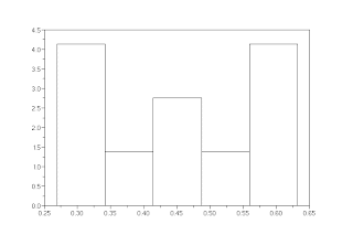
then you can see the histogram using the histplot(.) function.

histplot(5, x); // the function takes the biggest and the smallest values, divides the interval in five parts (the number 5, first argument), and counts how many numbers are in each part


Look the result:


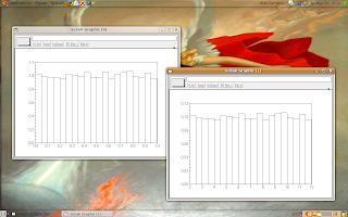
Now, let's do a smarter example:

x = rand(10000, 1);

y = 10*x + 2;

histplot(20, x);

scf(); histplot(20, y);


Look the result:


The graphs look like the same, but if you click over the image then you can see the indexes.

The left graph (variable x) has the indexes in the interval [0, 1] and the right graph (variable y) has the indexes in the interval [2, 12].

I ask to my readers: why the indexes are these?

Monday, August 17, 2009

Convolution

I wrote a post about convolution in my other blog, but I'll write here how to use the convolution in Scilab.

The convolution is a operation with two functions defined as:


The function in Scilab that implements the convolution is convol(.).

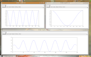
Let's do the test: I'll convolve a cosine (five periods) with itself (one period):

N1 = 100;
N2 = 20;

n1 = 1:N1;
n2 = 1:N2;

w = %pi/10;

f1 = cos(w*n1);
f2 = cos(w*n2);

y = convol(f1, f2);

plot(f1);
scf(); plot(f2);
scf(); plot(y);

The result is:

The top left graph is f1, the top right is f2 and the bottom graph is y.

Again, if anyone wants, I can write about discrete convolution properties.

Monday, August 10, 2009

FFT - specifying the frequencies

I'd like to know my readers, but the "no name" readers deserve respect, as everybody.

This post is about the FFT function, and anyone wants to know how to specify the frequencies for plot the values.

A few of theory:

If your signal has N values [0, N - 1], then the Fourier Transform has N distinct values.

The function fft(.) returns the signal in the interval [0, N - 1], so you can use the function fftshift(.), over the function fft(.) like this: X = fftshift(fft(x)), that it returns the Fourier Transform in the intervals:

  • [-(N - 1)/2, (N - 1)/2], if N is odd.
  • [-N/2, N/2 - 1], if N is even.

About the frequencies, if your signal was sampled with a rate T (T samples by second), the indexes are given multiplying the interval by: 2*%pi*T.

Look the example:

N = 100;

n = 1:N;

T = 0.1; // one sample by each 0.1s

w = 0.5; // frequency of the sampled signal (in radians)

x = cos(w*n);

plot(n*T, x); // plot the signal indexed by seconds

f = [-N/2:N/2 - 1];

X = fftshift(fft(x));

scf();
plot(f*2*%pi*T, X); // plot the signal indexed by radians


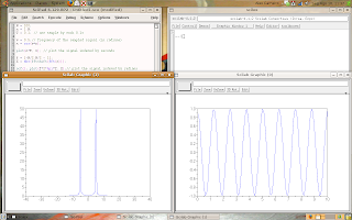
The result is:


Observing that w = 0.5 is the frequency of the sampled signal, the true frequency (of the analog source signal) is given by w_source = w/T = 0.5/0.1 = 5 rad/s. Now, click on the image and look where the peaks are.

Wednesday, August 5, 2009

Making functions

A important resource in any programming language is to make specific functions.
Using Scilab we may make our own functions.

For example, if we need a function that adds two numbers and divides the result by two, we can call that function as add_d2(v1, v2).

The follow script is made in the editor.


function [result] = add_d2(v1, v2)
aux = v1 + v2;
result = aux/2;
endfunction;


Or, we can write just one line of code:


function [result] = add_d2(v1, v2)
result = (v1 + v2)/2;
endfunction;


Obvious, the example is too simple, but I'd like to give a example for present the syntax.

Ok, let's make a better example:

We need a function that finds the peaks in a signal and returns two variable, one with the position and the other with the value of each peak.


function [positions, values] = find_peaks(x)
positions = [];
values = [];

n_peaks = 0;
for i = 2:length(x) - 1, // x should be a vector, like: x = [x_1 x_2 x_3 ... x_n]
if (x(i) > x(i - 1)) & (x(i) > x(i + 1)),
n_peaks = n_peaks + 1;
positions(n_peaks) = i;
values(n_peaks) = x(i);
end;
end;
endfunction;


Test the code and say me what happens.

Saturday, August 1, 2009

Fast Fourier Transform - FFT

This post is about a good subject in many areas of engineering and informatics: the Fourier Transform. The continuous Fourier Transform is defined as:


f(t) is a continuous function and F(w) is the Fourier Transform of f(t).

But, the computers don't work with continuous functions, so we should use the discrete form of the Fourier Transform:


f[n] is a discrete function of N elements, F[p] is a discrete and periodic function of period N, so we calculate just N (0 to N - 1) elements for F[p].

Who studies digital signal processing or instrumentation and control knows the utilities of this equation.

Now, how to use the Fourier Transform in Scilab?

If we are using large signals, like audio files, the discrete Fourier Transform is not a good idea, then we can use the fast Fourier Transform (used with discrete signals), look the script:

-->N = 100; // number of elements of the signal

-->n = 0:N - 1;

-->w1 = %pi/5; // 1st frequency

-->w2 = %pi/10; // 2nd frequency

-->s1 = cos(w1*n); // 1st component of the signal

-->s2 = cos(w2*n); // 2nd component of the signal

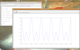
-->f = s1 + s2; // signal

-->plot(n, f);


The result is:


Now, let's study the Fourier Transform of our signal.

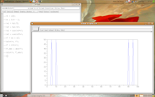
-->F = fft(f); // it calculates the Fourier Transform

-->F_abs = abs(F); // F_abs is the absolute value of each element of F

-->plot(n, F_abs);


The result is:


Look at the two graph's peaks, one for the component s1 and the other for the component s2.

The Fourier Transform is a linear transformation, thus it has a inverse transformation: the Inverse Fourier Transform.

Scilab has the function ifft(.) for obtain the original signal from it Fourier Transform.

If anyone wants to know, I can make a new post about how to identify the frequencies of the original signal in the Fourier Transform.