Tuesday, October 27, 2009

Response in frequency

Hi Cek, I saw your comment (here), and I'd like to say that I never worked with these functions before. But we can learn about the functions.

Let's start with the freq(.) function.

This code is the example in Scilab's help.


s = poly(0, 's');
sys = (s+1)/(s^3-5*s+4);
rep = freq(sys("num"), sys("den"), [0,0.9,1.1,2,3,10,20]);
[horner(sys, 0), horner(sys, 20)]
//
Sys = tf2ss(sys);
[A, B, C, D] = abcd(Sys);
freq(A, B, C, [0, 0.9, 1.1, 2, 3, 10, 20])


In the code, we see the function freq(.) is used with polynomials (in the Space of Laplace). The last argument (the vector [0, 0.9, 1.1, 2, 3, 10, 20]) represents the calculated frequencies for the polynomial sys.

The function tf2ss(.) means time/frequency to state-space.

The function refreq(.) does the same things of the function freq(.), but it uses other arguments.

Look the function's description, in Scilab's help.

[ [frq,] repf] = repfreq(sys, fmin, fmax [, step])
[ [frq,] repf] = repfreq(sys [, frq])
[ frq, repf, splitf] = repfreq(sys, fmin, fmax [, step])
[ frq, repf, splitf] = repfreq(sys [, frq])

Parameters

sys: syslin list : SIMO linear system
fmin, fmax: two real numbers (lower and upper frequency bounds)
frq: real vector of frequencies (Hz)
step: logarithmic discretization step
splitf: vector of indexes of critical frequencies.
repf: vector of the complex frequency response


The function horner(.) evaluates a polynomial in a specific point, for example:

s = poly(0,'s');
M = [s, 1/s]; // M is the polynomial in analysis
x1 = horner(M,1)
x1
x1 =

1. 1.

x2 = horner(M,%i)
x2 =

i - i

x3 = horner(M,1/s)
x3 =

1 s
- -
s 1


If you want, then we can try to learn anything about the others functions: bode, syslin and csim.
Friday, October 23, 2009

Operations element by element, again

Hi Jackmatze, how are you? I think you are just as old as me, but it's other thing.
About your question, I made a post that answers you: it's here.

So, let me show an example:

-->matrix1 = [1 2 1;
-->2 1 2;
-->1 2 3]
matrix1 =

1. 2. 1.
2. 1. 2.
1. 2. 3.

-->matrix2 = [1 1 2;
-->0 2 1;
-->1 3 1]
matrix2 =

1. 1. 2.
0. 2. 1.
1. 3. 1.

-->matrix_t = matrix1*matrix2
matrix_t =

2. 8. 5.
4. 10. 7.
4. 14. 7.

-->matrix_dott = matrix1.*matrix2
matrix_dott =

1. 2. 2.
0. 2. 2.
1. 6. 3.


Now, what's the difference of matrix1^2 and matrix1.^2?

matrix1^2 = matrix1*matrix1

matrix1.^2 = matrix1.*matrix1


Ok, Jack? Anything more, I'll try to help you.

Peaks in FFT transformation

Hi Kaustubh, excuse me for the time of the answer.

Do you want to know about the peaks in the FFT transformation (here), right?

Well, this blog is about Scilab, and you can find what you want in any book of Digital Signal Processing.

But God loves you and I'll try to explain what the peaks mean.

Think in a pure frequency signal x(t) like a sine or cosine, it has only the own frequency (f0). The FFT transform is two impulses (X(f) = d(-f0) + d(f0)) (similar to this figure)

If you plot the FFT transform of x(t), then you obtain the peaks in -f0 and f0.

Now, think in a signal composed by two pure frequency signals, y(t) = x1(t) + x2(t), of different frequencies (f1 and f2).

The FFT transform of y(t) is four impulses, two for x1(t) and two for x2(t).

If x1(t) and x2(t) have different amplitudes, for example: x1(t) = cos(2t) and x2(t) = 3 cos(5t), then the peaks of the FFT transform of y(t) are weighted,

Following the example, the FFT transform of x1(t) is X1(f) = d(-f1) + d(f1) and the FFT transformation of x2(t) is X2(t) = 3(d(-f2) + d(f2)). So, the FFT transform of y(t) = x1(t) + x2(t) is Y(f) = X1(f) + X2(f) = (d(-f1) + d(f1)) + 3(d(-f2) + d(f2)).


Now, if you have a real signal xr(t), it has many frequencies and it FFT transform XR(f) presents many peaks, one by each frequency. The peaks' amplitude represents the amplitude of each frequency in xr(t).

My friend, I said this not a blog about Signal Processing, but I tried to help you.
If you have more question, I'll try to help you again.

Tuesday, October 20, 2009

Tensors

Hi Michele, how are you?

First, I'm sorry because I'm not an expert in multi linear algebra and I don't know many things about tensors.

In a fast search, I saw tensors are like matrices with high dimensionality.

Correct me if I were wrong.


tensor1 = zeros(3, 3, 3); // it's a tensor

tensor2 = ones(5, 5, 4); // it's other tensor


I found one function that works with tensors: kron(.). It returns the Kronecker tensor product of two matrices A and B.

The function kron(.) is called like following:


A=[1,2;3,4];

kron(A,A)
ans =

1. 2. 2. 4.
3. 4. 6. 8.
3. 6. 4. 8.
9. 12. 12. 16.

A.*.A // this operator (.*.) implements the Kronecker tensor product of two matrices, look the results are the same kron(A, A) == A.*.A
ans =

1. 2. 2. 4.
3. 4. 6. 8.
3. 6. 4. 8.
9. 12. 12. 16.


I think it's something about tensors.
If anyone has a comment or suggestion, I ask for you share your knowledge with us.

Thursday, October 8, 2009

Topics of Digital Image Processing

Hi Wahlau, I saw your comment but I couldn't answer it before. Thank you for your words to me.

I have another blog and I made some posts about Image Processing and Segmentation (in Portuguese).

If you want to develop anything like the interactive ball, then you should learn about skin segmentation and how to interact the virtual ball with the segmented region.

The simplest algorithm for skin segmentation is the threshold in the channels of color Cb and Cr (in images coded in YCbCr).

The toolbox SIVp has functions for read, write, show, convert, and others operations with images. That toolbox is too simple for install, if you use GNU/Linux, you can install it using the apt-get or synaptic.


PS.: In my other blog, I posted some codes in Scilab for skin segmentation, and anything more.

Tuesday, October 6, 2009

Excuses

Hi Stanley and Naza, I'm sorry I couldn't answer your questions because I'm writing my dissertation and I needed to make two articles too.

So, I ask for you explain better what you want.

Stanley, I think the meshgrid() function can help you, like following:

N = 20;
x_range = -1:2/(N - 1):1;
y_range = -1:1.2/(N - 1):0.2;

[x y] = meshgrid(x_range, y_range);

P = [];
for i1 = 1:N,
for i2 = 1:N,
P(i2,i1) = color_P(i1, i2); //here you put the function P = f(x, y)
end;
end;


---------------

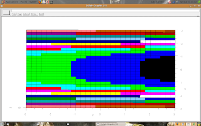
For plot the graph, you can use the fplot3d1(.) function. The following picture shows a example:

deff('z=f(x,y)','z=x^4-y')

x=-3:0.2:3 ;y=x ;

fplot3d1(x, y, f, alpha = 0, theta = 0); // alpha and theta are the rotation angles


The result is:


Now, you study the fplot3d1(.) function for make your own graph.

The presented function plots graphs as surfaces if you change the variables alpha and theta (try alpha = 5 and theta = 30).

That's all.

Thursday, October 1, 2009

Digital Signal Processing - intro

Hi Wallace, I'd like to know what algorithm, or kind of algorithm, you need to develop.

I made a post about convolution, but I think it's a good, and simple, subject for we start our studies.

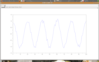
Look the noised signal:

-->T = 100;

-->t = 1:T;

-->w = %pi/10;

-->s = cos(w*t); //pure signal

-->n = rand(1, T, 'normal')*0.1; //noise

-->x = s + n;

-->plot(t, x);


The result is:


Now, let's filter the signal using an average filter.

We have two options for apply the filtering:


The first

-->Tm = 5;

-->y = [];

-->for i = 1:Tm,
-->y(i) = mean(x(1:i));
-->end;

-->for i = (Tm + 1):T,
-->y(i) = mean(x((i - Tm):i));
-->end;

-->plot(t, y);


The result is:


The second

-->Tm = 5;

-->m = ones(1, Tm);

-->y = convol(x, m);

-->ty = 1:length(y);

-->plot(ty, y);


The result is:


If you make the math operations, you'll see the results are, numerically, the same for t = Tm + 1 until t = T.