Wednesday, November 6, 2013

Parsing string to math expression with inline function

This week, I discovered a new math game for Android: Match The Math (https://play.google.com/store/apps/details?id=com.engcross.matchthemath).

I have seen this app converts a string to a math expression and solves it in real-time. So I though about how doing it in Scilab, to get a string like "2*5 + 2" and return the number that corresponds to the result of the expression, in the example 12 (= 2*5 + 2).

Scilab has an interesting way to create "one line" functions, e. g. sum2numbers(a,b) where this function should return just a+b. This way is called inline functions and is defined like following:

deff('[x]=func(a,b)', 'x=a+b');

Where '[x]=func(a,b)' defines the structure of the function with x being the return, func is the name of the function and a and b are the arguments; 'x=a+b' is what the function executes when is called: x=a+b.

With this concept in mind, we can use a inline function to parse a string to a arithmetic expression because deff() uses only strings as arguments.

Let's use a common function definition, with a string to be parsed as argument, and one inline function inside:

function [x]=parsingStr2Arithmetics(s) // definition of the function
deff('[x]=f()', 'x='+s); // creates inline function that parses the string
x = f(); // calls the function to return it result
endfunction; //end of the function


Now our function is ready, we can test it using different expressions as arguments.

-->parsingStr2Arithmetics("2")
 ans  =

    2. 

-->parsingStr2Arithmetics("2+2")
 ans  =

    4. 

-->parsingStr2Arithmetics("2+2*5")
 ans  =

    12. 
-->parsingStr2Arithmetics("(2+2)*5")
 ans  =

    20. 

-->parsingStr2Arithmetics("(2+2)*5 - 3")
 ans  =

    17. 


For finishing this post, I recommend you to try Match The Math game, it's really cool and improves our math and problems solving skills.

Tuesday, October 8, 2013

Scilab as supporting software for mobile

In Eng Cross' blog we can see some apps those have Computer Vision features. I have known OpenCV, Open Computer Vision API, has a wrapper for Android, which is used by Eng Cross in his apps.

Nowadays, there are information about two apps:

4 Views

This app applies four different effects in camera's image and composes a new image where the user can select one effect to be applied to the image and save pictures in Pictures directory.


Right Angle

This app creates a "L" mark in the center of the screen and identifies any right angle aligned with the mark holding the screen and pointing the vertex of the angle.


But, what's the relation between these Android apps with Scilab?

Scilab has the toolbox SIVp (Scilab Image and Video Processing toolbox) that can be used for testing similar algorithms. Once developing codes in Scilab is much faster than in any programming language, it's very useful to use this simulation environment for making first tests and validations of advanced algorithms, like computer vision, image/signal processing, statistics analysis, math modeling, etc.

Added to being an simulation environment, Scilab can work as server for high intensive processing solutions, concentrating information, e. g. from sensors, and sharing data to mobile devices through webservices, like using JSON.

Wednesday, August 14, 2013

JSON in Scilab

Hi dears, today I've met a tool for Scilab that makes possible to handle JSON files into Scilab code. This tool is available through ATOMS or in http://forge.scilab.org/index.php/p/json/

Once installed, let's make a simple test with this tool just for validation.

First, it's created a json file (json_test.json) like below:

{
  "orderID": 12345,
  "softwareName": "Scilab",
  "ToolName": "JSon",
  "contents": [
    {
      "productID": 1,
      "productName": "Test1",
      "quantity": 1
    },
    {
      "productID": 2,
      "productName": "Test2",
      "quantity": 3
    }
  ],
  "demoCompleted": true
}


Now, it's needed to get this file into Scilab, what we can do uding mgetl(.) function:

json_test = mgetl("file_test.json");

Take attention for the path of the file.

And the function JSONParse(.) returns the struct that corresponds to the data in the file, like this:

mystruct = JSONParse(json_test)

The expected result is

-->mystruct
 mystruct  =

   orderID: 12345
   softwareName: "Scilab"
   ToolName: "JSon"
   contents: [1x2 struct]
   demoCompleted: "%T"


For accessing the fields, try this:

-->mystruct.orderID
 ans  =

    12345. 

-->mystruct.ToolName
 ans  =

 JSon  

-->mystruct.contents.productName
 ans  =


       ans(1)

 Test1  

       ans(2)

 Test2  


JSON is like XML pattern, much used for WebServices and in other Internet cases. Thus, I recommend to spend a few time taking a look about this technology and how Scilab can aggregate value to your solutions.

Monday, July 1, 2013

Plotting conical curves - circles

Conical curves are very known geometric spaces based on section of cones. There are four conical curves:
  • circle;
  • ellipse;
  • hyperbole;
  • parabola.

All of them are very used in computer graphics and, in this post, I wish to present how to plot a circle.

The analytic equation of circles is: (x - xc)² + (y - yc)² = r² where (xc, yc) means the center of the circle and r is it radius.

We know cos²(a) + sin²(a) = 1, for any angle a, thus multiplying both sides of equation by we obtain (r cos(a))² + (r sin(a))² = r².

Comparing original equation with obtained equation, it's possible to verify that:

x - xc = r cos (a)
x = r cos(a) + xc

y - yc = r sin(a)
y = r sin(a) + yc


So, we have now the values for x and y depending only of the center of the circle, it radius and an angle a.

(xc, yc) and r are given by the circle and a is an angle that means a dummy variable in range [0, 2*%pi].


Now, let's write some code in Scilab.

By first, a circle of radius r = 2 and center (xc, yc) = (0, 0).


//center of the circle
xc = 0;
yc = 0;

//radius of the circle
r = 2;

//dummy variable for angle in range [0, 2*%pi]
a = linspace(0, 2*%pi, 100);

//x axis
x = xc + r*cos(a);

//y axis
y = yc + r*sin(a);

//plot the circle
plot(x, y);


The result of this code is the following picture.

Take attention the limits of the circle are (-2, 2) both for x and y axis, what means this circle is centered in (0,0) with radius 2.


And for finishing, a harder example, four circles with different centers and radius.

/////////////////////////////////////////
//center of the circle
xc = 6;
yc = 0;

//radius of the circle
r = 6;

//dummy variable for angle in range [0, 2*%pi]
a = linspace(0, 2*%pi, 100);

//x axis
x = xc + r*cos(a);

//y axis
y = yc + r*sin(a);

//plot the circle
plot(x, y);

////////////////////////////////////////
//center of the circle
xc = 6;
yc = 0;

//radius of the circle
r = 2;

//dummy variable for angle in range [0, 2*%pi]
a = linspace(0, 2*%pi, 100);

//x axis
x = xc + r*cos(a);

//y axis
y = yc + r*sin(a);

//plot the circle
plot(x, y);

////////////////////////////////////////
//center of the circle
xc = 2;
yc = 0;

//radius of the circle
r = 2;

//dummy variable for angle in range [0, 2*%pi]
a = linspace(0, 2*%pi, 100);

//x axis
x = xc + r*cos(a);

//y axis
y = yc + r*sin(a);

//plot the circle
plot(x, y);

////////////////////////////////////////
//center of the circle
xc = -3;
yc = 3;

//radius of the circle
r = 3;

//dummy variable for angle in range [0, 2*%pi]
a = linspace(0, 2*%pi, 100);

//x axis
x = xc + r*cos(a);

//y axis
y = yc + r*sin(a);

//plot the circle
plot(x, y);

And the result is:


Take attention the parameters of center and radius of each circle and the obtained picture.

Tuesday, April 9, 2013

Analytical derivation with Scilab

Today, I have discovered one useful function in Scilab, the derivat() function that works with expressions like
which consists of functions of linear combinations with integer exponents of one variable (in the example denoted by z).

The function derivat() implements the analytical derivation of p(z), giving the following result:

We can create this kind of expression with Scilab function poly(), like this:
-->p1 = poly([1 -2 1], 'x', 'coef')
 p1  =

                   2 
    1 - 2x + x  

-->p2 = poly([1 -4 2], 'y', 'coef')
 p2  =

                     2 
    1 - 4y + 2y  

-->p3 = poly(ones(1, 10), 'z', 'coef')
 p3  =

                 2    3    4    5    6    7    8    9 
    1 + z + z + z + z + z + z + z + z + z   

-->p4 = poly([-1 1], 't', 'roots')
 p4  =

           2 
  - 1 + t

-->s = %s; p5 = s^{-1} + 2 + 3*s
 p5  =

                     2 
    1 + 2s + 3s  
    -----------  
           s       


And so on.


Now, the derivat() function implements the analytical derivation of the given functions:

-->derivat(p1)
 ans  =

  - 2 + 2x  

-->derivat(p2)
 ans  =

  - 4 + 4y  

-->derivat(p3)
 ans  =

                    2      3      4      5      6      7      8 
    1 + 2z + 3z + 4z + 5z + 6z + 7z + 8z + 9z  

-->derivat(p4)
 ans  =

    2t  

-->derivat(p5)
 ans  =

             2 
  - 1 + 3s  
    ------  
       2    
      s     


There is a way for applying your knowledge about linear systems with a powerful open source simulation tool.

Thursday, April 4, 2013

Creation of artifical data for classification tests

In this semester, I'm teaching Artificial Intelligence discipline, and we are studying algorithms of classifying: Decision Trees and Neural Networks.

One important task of the discipline is to test the developed algorithm and estimate it accuracy. For that, I use to create artificial data which is controlled and simple to analyze.

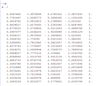
The data consists of one table of N columns and many rows (let's use M rows). N - 1 first ones columns are of input data and the last column means the label (target), like presented below.

The variable x presented is a matrix (table) with 5 columns and 20 rows. Being 4 columns of input data and the last column a label for each row.

Label data are in a subset of natural numbers {1, 2, 3, 4, ....}, in the presented case {1, 2} where 1 means one class and 2 means the other.

N - 1 first columns are created through rand() function using M/P rows for each class of data, with it we created a equal distributed data set for classes representativeness (P means how many classes are in the data set).

For the variable x presented, it was created like following.

-->n = 10;

-->x = [[rand(n, 1); rand(n, 1) + 0.9] [1 + 2*rand(n, 1); rand(n, 1)*0.5 + 0.65] [rand(n, 1, "normal"); rand(n, 1) + 2.5] [rand(n, 1, "normal") - 2; rand(n, 1, "normal") + 2] [ones(n, 1); 2*ones(n, 1)]];

But it's possible to use only simpler forms of combined columns for creating overlapped input data.

Once created the matrix, we can write it to a file:

-->write("my_data.txt", x);


And later we can read the data again to a variable:

-->y = read("my_data.txt", -1, N);

Take a look at

http://usingscilab.blogspot.com.br/2009/03/using-files.html

http://usingscilab.blogspot.com.br/2009/08/basic-statistic.html

http://usingscilab.blogspot.com.br/2011/02/statistics-operators-mean-and-stdev.html

http://usingscilab.blogspot.com.br/search/label/matrix

for more details.


Monday, February 4, 2013

2D Rotation

Let's make a rotation of a square. First, we create the square:

A = [0, 0];

B = [1, 0];

C = [1, 1];

D = [0, 1];

sq = [A;
      B;
      C;
      D;
      A];

plot2d(sq(:,1), sq(:,2), rect = [-.1 -.1 1.1 1.1]);

The result is the following picture.


For rotating this object an angle a = pi/4 (45°), we can do

a = %pi/4;

r = [cos(a) -sin(a);
     sin(a) cos(a)];

sq_r = sq*r;

plot2d(sq_r(:,1), sq_r(:,2));

 The result is


The same technique can be done for rotation any kind of geometric structure.

For another example, look a random structure and its rotation.

sq = rand(10, 2);

plot2d(sq(:,1), sq(:,2), rect = [-.1 -.1 1.1 1.1]);

a = %pi/4;

r = [cos(a) -sin(a);
     sin(a) cos(a)];

sq_r = sq*r;

plot2d(sq_r(:,1), sq_r(:,2), style = 2);


The result is

Take attention the presented rotation method rotates the object using the center of axes (point (0, 0)) as reference. However, it's very simple to change the point of reference just adjusting matrix r, can you do this?


Wednesday, January 23, 2013

Equalis Introduces Advanced Image and Video Processing Module - Equalis - Where Engineering and Science Computes

Equalis Introduces Advanced Image and Video Processing Module - Equalis - Where Engineering and Science Computes

This a very interesting new for engineers, students and researchers who work with image processing and/or computer vision, like me.

I hope to study something about this new module soon and I can support anyone else that intend to begin in this amazing area.

Happy year of 2013 for everyone!